Ten recommendations for scanning foraminifera by X-ray computed tomography

Marine sediment cores uniquely provide a temporally high-resolution and well-preserved archive of foraminifera fossils, which are essential for understanding environmental, ecological, and evolutionary dynamics over geological timescales. Foraminifera preserve their entire ontogeny in their fossilized shells, and much of this life history remains hidden from view under a light microscope. X-ray microfocus computed tomography (μCT) imaging of individual foraminifera reveals internal chambers and pores that are traditionally hidden from view. Their volume, shape, and growth form foundations of oceanographic and environmental research.

Here, we present a set of 10 recommendations for the preparation and scanning of individual fossilized foraminifera using glue-, gel-, and solvent-free methods. We focus on the primary X-ray parameters of μCT imaging that a researcher can optimize according to their throughput, signal-to-noise ratio, and cost requirements to generate three-dimensional (3D; volumetric) datasets. We showcase the effect of these parameters on image quality through repeated scans on a single planktonic foraminifer that varied the X-ray beam power and energy, detector binning, number of projections, and exposure times.

In our case study, the highest beam power resulted in the widest contrast between the subject of interest and the background, allowing the easiest threshold-based segmentation of the object and aiding computers in automated feature extraction.

The values of these parameters can exhibit significant variability across individuals, based on the specific needs of the study, the equipment used, and the unique attributes of the samples under consideration. Our motivation with this paper is to share our experience and offer a foundation for similar studies.

1 Introduction

X-ray microfocus computed tomography (μCT) is a popular, non-destructive technique to study internal structures and features hidden from external view. High-quality images are convenient for manual analysis of internal morphology that has long been associated with forensic evolutionary divergence (Huber et al., 1997; de Vargas et al., 1999). In recent times, these images are valuable inputs for training machine learning and image classification tools, which are being developed to automate species identification, feature identification, and quantification of key taxonomic features (Mulqueeney et al., 2024; Marchant et al., 2020; Hsiang et al., 2019).

X-ray CT is powerful three-dimensional (3D) imaging technology that opens new horizons for understanding environmental, ecological and evolutionary dynamics by revealing internal views compared to the surface level of traditional light microscopy. High-resolution microfocus X-ray CT (μCT) imaging, 3D reconstruction algorithms, and volume data analysis software enable researchers to quantify morphological changes at both intra- and interspecific intervals (Caromel et al., 2016; Burke et al., 2020; Schmidt et al., 2013), extract ontogenetic trajectories, identify the extent of dissolution (Johnstone et al., 2010; Iwasaki et al., 2015), measure shell wall thicknesses as a proxy for dissolution, and correlate changing geochemical signals with subspecies taxonomic variation (Kearns et al., 2023), all without damaging the specimens.

Fossilized foraminifera tests preserve the individual organism's entire ontogeny alongside the environmental conditions during the period of calcification. Brummer et al. (1987) describe the five stages of foraminifera growth from the proloculus through the juvenile and neanic stages before maturing in the terminal reproduction stage. Using X-ray CT and post-processing software, researchers can calculate chamber growth rates and aspect ratios as one technique to identify when ontogenetic transitions occur, especially in the earlier chambers that are hidden from a traditional light microscope view. Computer software packages aid the quantification of three-dimensional growth trajectories using chamber centroid coordinates and can be applied quickly across large datasets. The resulting 3D models are also useful teaching aids that show in detail the wall texture, porosity, and every grown chamber that Brummer described.

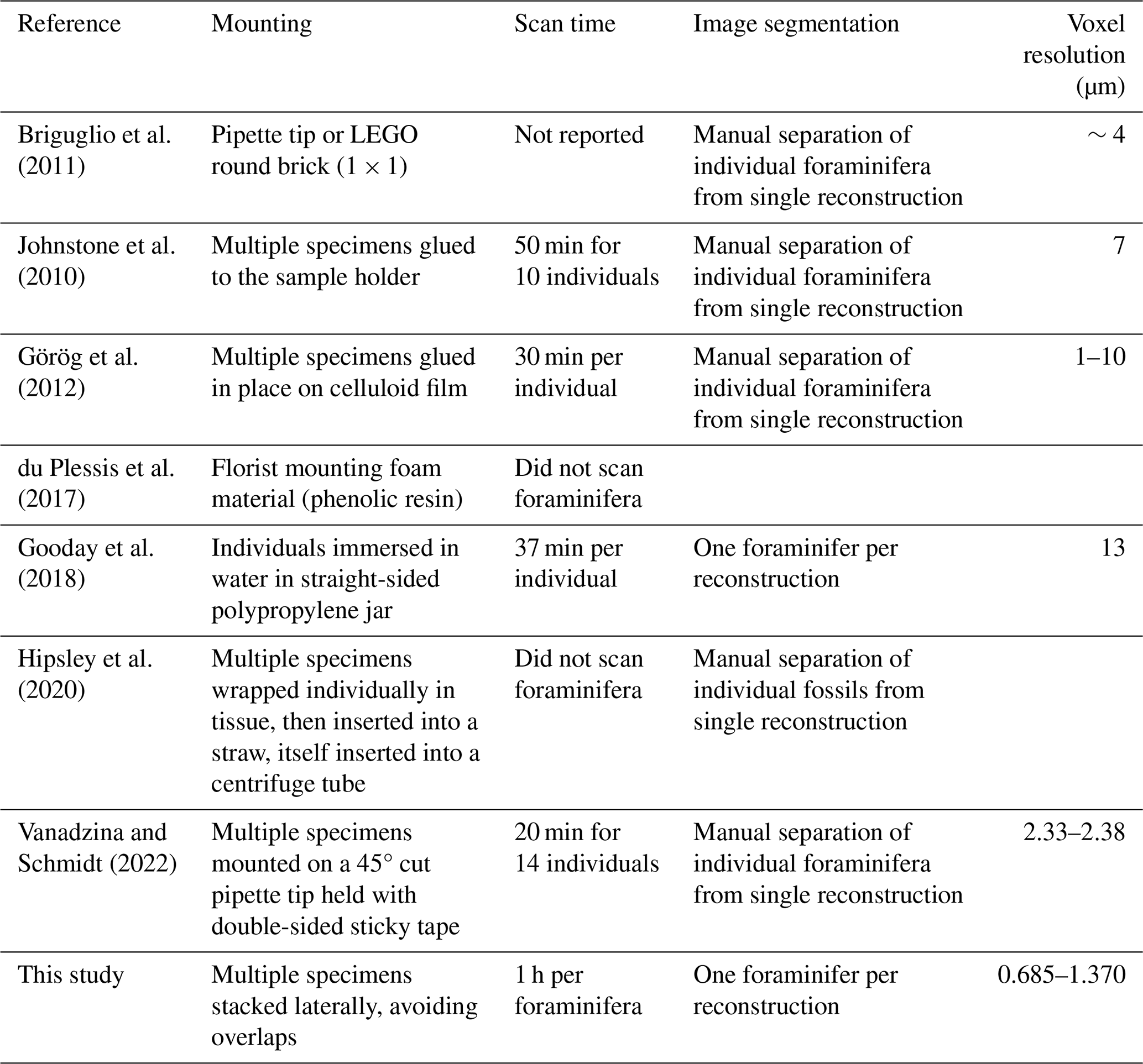
Various methods of sample preparations for scanning and the corresponding scanner configurations have been described (Görög et al., 2012; Hipsley et al., 2020; du Plessis et al., 2017; Briguglio et al., 2011; Vanadzina and Schmidt, 2022; Johnstone et al., 2010; Gooday et al., 2018). Methods in the literature include mounting foraminifer specimens on individual wooden toothpicks or pipette tips (Kendall et al., 2020; Vanadzina and Schmidt, 2022), keeping the specimen exposed to surroundings and dust and increasing the risk of loss. Table 1 compares the sample mounting methods, the time taken to scan, the post-reconstruction segmentation of individual foraminifera, and the achieved resolution of benchtop X-ray CT setups for these references that used laboratory benchtop instrumentation.

Table 1 Comparisons for mounting methods, the time taken to scan, the post-reconstruction segmentation of individual specimens, and the achieved resolution of benchtop X-ray CT setups for scanning foraminifera where available.

Here, we present 10 recommendations to optimize the throughput of X-ray computed tomographic scanning of planktic foraminifera. One of these recommendations is a sample mounting method which does not include glue, gel, or solvents that could interfere with accurate image segmentation, facilitating structured data storage and resulting in a relational database. In our case study, woven throughout this article, we housed 20 foraminifera encased within malleable phenolic resin foam (florist mounting foam) within a rigid plastic straw, isolating the samples from dust and making an easily transportable unit without the risk of losing the specimens.

Similar principles are applicable to other fossils (e.g. other protist shells, coral fragments, and otoliths) that researchers may need to scan using a laboratory-based X-ray CT setup. Our method presents a standardized operating procedure for micro-CT analysis that is advantageous for research projects that contain more individual specimens than can be scanned in a single session and prioritizes consistency within and between scanning sessions. From the case study we present here, the resulting data facilitate greater reproducibility and reusability in collaboration amongst the morphologically and geochemically inclined members of the micropalaeontological community.

2 Laboratory CT scanning

Laboratory X-ray micro-CT scanners function by emitting a focused X-ray beam through a specimen to a detector. X-rays are generated when a heated cathode filament ejects electrons that accelerate and hit a tungsten anode, producing X-ray photons through bremsstrahlung radiation or characteristic emission. The X-ray beam passes through the specimen, with attenuation proportional to the sample's density, and is measured by the detector, which translates the energy into greyscale values reflecting density variations. In a benchtop setup, the X-ray source and detector are fixed, while the specimen rotates incrementally, capturing two-dimensional (2D) projections from various angles. These projections are then back-projected and processed to reconstruct a 3D volume. Geometric magnification, influenced by the distances between the X-ray source, specimen, and detector, affects image resolution, with small focal spots minimizing geometric blurring.

We used a ZEISS Xradia 510 Versa X-ray micro-CT benchtop scanner in the case study presented here. The X-ray beam was pre-filtered through a 0.15 mm SiO₂ ceramic filter to absorb and attenuate the lower-energy X-ray photons from the spectrum, resulting in a beam that is enriched with higher-energy photons, improving the contrast and reducing beam-hardening artefacts in the final image as discussed below. This instrument features a two-stage magnification: the sample is enlarged through geometric magnification, then the beam hits a scintillator that converts X-rays into visible light, which is then magnified through an optical lens. This visible light then hits the detector, and a projection is recorded. This setup enabled us to achieve a spatial resolution of 990 nm, which is detailed enough to resolve the smallest of chambers and higher than would have been possible on a benchtop CT scanner without the second magnification stage. The Versa system was a more costly option than simpler benchtop laboratory CT-scanners but less expensive than synchrotron time.

3 The 10 recommendations

3.1 Preparation

3.1.1 Specimen selection and cleaning

Selecting which specimens to scan can take some consideration. As dissolution starts at the smallest internal chambers of a foraminifer, it may not be possible to judge the preservation state before taking the scan (Johnstone et al., 2010; Iwasaki et al., 2015). If the study is to research well-preserved foraminifera, we suggest selecting a larger number of individuals to have enough non-dissolved specimens. The loss of internal septa (dividing walls between chambers) hinders chamber identification, which reduces the usefulness of the scan data for studying their life history. Stratified random sampling within a “best-preservation” category will facilitate representative environment, ecological, and evolutionary interpretations of the data.

This is the stage to check the specimen is free from surface debris and embedded particulates. In our case study, we followed the ultrasonication in ethanol method described in Eggins et al. (2003).

Identifying each individual specimen throughout the process from selection through scanning to data processing requires a systematic naming scheme to assign unique identifiers and a database, which can be as simple as a spreadsheet.

3.1.2 Mounting in a straw

Our method suggests mounting specimens in a single vertical stack within a rigid, clear plastic drinking straw encased within malleable phenolic resin foam (florist mounting foam), isolating the sample from dust and making an easily transportable unit (Figs. 1 and 2). The straw and foam keep the specimen securely in place during scanning, which is essential for collecting high-quality scans and is readily removed in post-processing due to the density difference between materials. Selecting a straw with the narrowest diameter that will accommodate the largest specimen will minimize the distance between the source beam and the specimen when mounted within the scanner, which will maximize geometric magnification of the specimen and beam intensity at the detector while also reducing the necessary image exposure time.

Figure 1 Our Xradia 510 Versa setup used throughout the presented case study. Key instrument parts shown are a tungsten X-ray source, a scintillator with optical magnification, and a charged coupled device (CCD) detector. The X-ray beam, shown as grey shading, passes through a 0.5 mm SiO₂ ceramic filter before entering a plastic straw packed with foraminifera sandwiched between green foam and with grey foam after every five specimens to build blocks of specimens and safe areas to cut for specimen retrieval and a blue marking to indicate the top of the straw to ensure the scan data correspond to the expected specimen. Individual specimens and each block are captioned in the figure. The straw is clamped to a stage and is incrementally rotated after each radiograph is taken. The box insert shows a schematic during the assembly of a straw by pushing individual foam slices with a pressed well containing a single foraminifer within the middle of the straw. Each foam slice is pushed up the straw until the slice meets the foam above, without crushing the foam, to maintain separation between individual specimens.

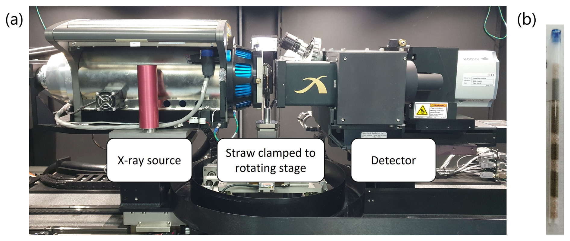
Figure 2 Case study setup showing (a) the X-ray source, a straw clamped to a rotating stage, and a scintillator with 4× optical magnification lens in front of the detector and (b) the same straw as constructed before clamping to the rotating stage, with the blue marking indicating the top of the straw.

In an example setup including 20 individual planktic foraminifera, where the diameter of the largest specimen is ∼1 mm, we selected a 2 mm diameter wide and 10 cm tall straw. A taller straw when clamped at the bottom may be less stable at the top, causing motion artefacts in the images of the highest mounted specimens. Using the empty straw, we pressed out a 2 mm diameter disc of grey foam to mark the top of the stack and used a rod with the same internal diameter as the straw to push this foam slice to about 1 cm from the top. Next, we marked a 2 mm diameter disc of green foam and made a small well in the centre of the disc to hold a specimen. The slices of green foam should be sufficiently thick that no two specimens will touch, as this can cause automated algorithms in the post-processing stage to misassign the specimen identifier with the scan data. A specimen is easier to retrieve from a thicker slice of foam after scanning, as there is more foam surface area to grip while removing the slice from the straw. The well in the foam slice should be in the middle so that, when the specimen is imaged in 360°, the centre of rotation is also in the middle. Having the centre of rotation in the middle of the straw narrows the field of view required by the detector, thereby reducing the number of radiograph projections required and consequently the time taken to scan the specimen. The well acts as a nest for the specimen but should be narrow enough to maintain a tight fit.

Once a specimen was transferred into the well, the slice was pushed up against the previous foam slice to secure the specimen in place. We repeated this process until there was a stack of five foraminifera making the first block. We then pressed a 2 mm disc of grey foam and pushed this up the straw to separate the end of the first block and the start of the second block. The slices of grey foam that separate the layers of green foam that make up the blocks are added, as they help the scanner operator navigate the straw under X-ray when locating the specimens during setup. In our example, the grey foam occurs after every five specimens, offering a secondary check that all five specimens in the block have been accounted for before progressing, and provides an area in the straw that is safe to cut after scanning to aid the retrieval of the specimens from the straw. By stacking the specimens vertically, the X-ray beam has only one specimen to pass through before reaching the detector, which reduces the opportunities for beam-hardening artefacts when compared to horizontal stacking.

We repeated building blocks of five foraminifera, separated by foam slices, until all 20 specimens had been loaded. Separating specimens like this facilitates keeping track of individuals using the location of each specimen within the straw and is an important detail in the relational database. We used a naming scheme that includes the straw number, the block number, and the foam slice number to identify each individual specimen. These unique identifiers aid the scan operator to locate individual specimens within a straw under X-ray and without the need of a visual map of each specimen location in the straw.

For continuity between scans, each specimen should be assigned its own tomography point and be the exclusive subject within it.

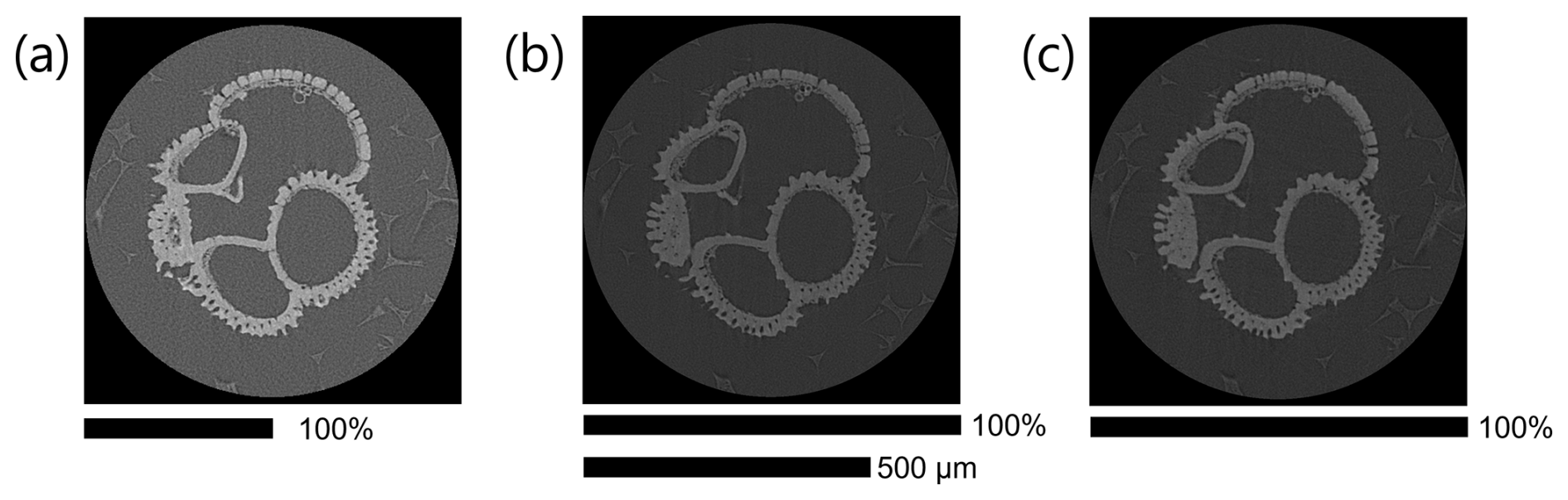
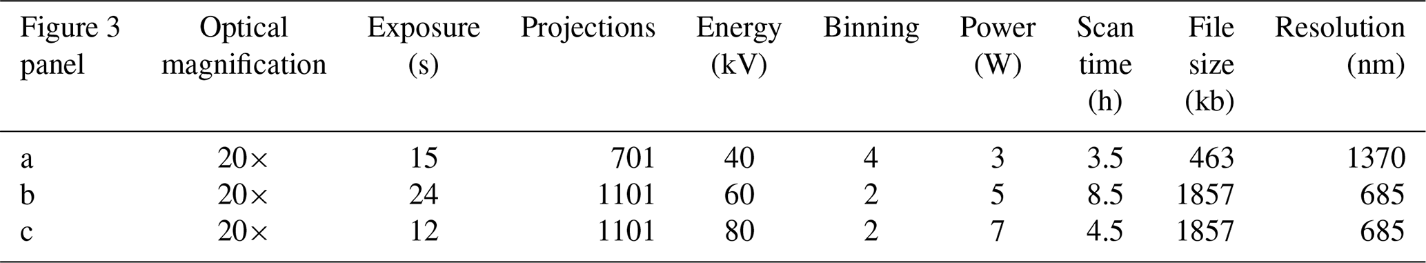
Figure 3 The same Dentoglobigerina altispira foraminifer was repeatedly scanned with varying parameters, and a single slice from the reconstructed .tiff stacks is presented to visually compare the effects of resolution, contrast, and artefacts. A scale bar shows the relative width of each square image and indicates that image (a) is presented twice as large to make the 500 µm scale bar applicable to all images. (a) 15 s exposure, 40 kV, and 4× binning achieving 1370 nm resolution; (b) 24 s exposure, 60 kV, and 2× binning achieving 685 nm resolution; (c) 12 s exposure, 80 kV, and 2× binning achieving 685 nm resolution.

3.2 Scanning parameters

3.2.1 Purpose of the study

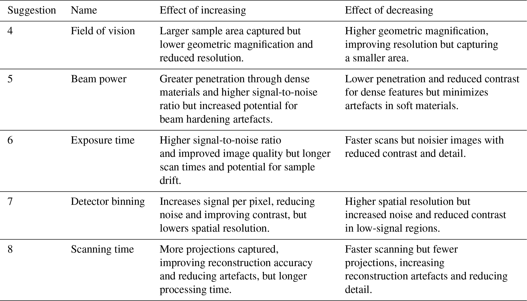
All the guidelines presented in this paper impact scanning time and the resulting image quality; this trade-off defines the optimization process.

The choice of scanning parameters is dependent on the purpose of the study. A large study with many individual specimens may prioritize minimizing the time taken for setup and scanning, encouraging an increased throughput. Other studies may prioritize image contrast, 3D volume resolution, or the standardization of parameters.

In our case study, we selected green and grey foams that both had lighter, but different, densities to the specimen to ensure a separation in greyscale values in the reconstructed images. A wider separation between specimen and support makes region-of-interest separation by grey value thresholding simpler during post-processing. Table 2 quantifies the effects of exposure time, the number of projections, the beam energy and power, and the amount of detector binning on the resulting radiographs (Fig. 3). We summarize the effects of increasing and decreasing each X-ray CT scanning parameter, as discussed in suggestions 4–8, in Table 4.

Table 2 Instrument parameters for repeated scans of a single Dentoglobigerina altispira foraminifer with the achieved resolution and resulting file size.

3.2.2 Field of vision

The highest spatial resolution is achieved by the specimen filling the detector's entire field of view. Filling the field of view is achieved by magnifying the specimen through a geometric magnification and, on Versa-like systems, an additional optical magnification stage. Filling the field of view utilizes more of the detector pixels to capture information from the specimen, contributing to a finer spatial sampling resulting in a detailed image and consequently a higher resolution.

Higher geometric magnification is achieved by decreasing the distance between the source and the specimen while increasing the distance between the specimen and the detector. Increasing the distance between the specimen and the detector provides a longer distance for the X-rays to diverge, leading to a larger area covered by the X-ray beam and greater magnification.

While widening the distance between the specimen and the detector increases magnification and spatial resolution, the image brightness reduces because the detected beam intensity is inversely proportional to the square of the distance from the source. To counter the reduced brightness caused by increased distance, the beam power could be increased, the exposure time could be lengthened to capture more X-rays, or greater detector binning could be applied to increase sensitivity.

By using more of the sensor to capture the foraminifera, there are fewer pixels to capture the surrounding foam or background noise, helping to enhance the signal-to-noise ratio and the selective allocation of pixels. The expanded coverage of the sensor by the foraminifera in each image facilitates enhanced artefact removal or reduction during 3D reconstruction, attributed to the increased number of overlapping pixels in each projection. Image artefacts that may occur because of undersampling and because of underutilizing the sensor include streaks, rings, and blurring of density boundaries (such as the edge of the denser foraminifer calcite and lower-attenuating foam).

By stacking specimens vertically within the plastic straw, we remove the horizontal overlapping of specimens and therefore the chance of beam hardening to occur, which can cause artefacts. By reducing the horizontal overlapping, greater magnification can be achieved to fill the field of vision, further increasing the spatial resolution. Avoiding the X-ray beam passing through multiple specimens in the same path reduces the chance of beam-hardening artefacts, which reduce image quality and can cause some automated 3D reconstructions to fail.

3.2.3 Beam power

Increasing the beam power emits more photons at a higher energy. Denser areas within the specimen cause more attenuation to the X-ray beam, so photons require greater energy to pass through these areas. Higher-energy photons penetrate the specimen further, resulting in higher detection intensity and less difference in attenuation between different parts of the specimen, which lead to lower contrast. A compromise between sufficient power to penetrate the densest area of the sample and sufficient contrast between regions of interest is needed to capture a useful radiograph. In our example of a foraminifer specimen (Fig. 3), the beam power was enough to penetrate the denser shell wall, while retaining enough contrast to separate the calcite test from the primary organic membrane layer and surrounding phenolic foam.

Benchtop X-ray CT sources often produce polychromatic X-ray beams, which contain a range of photon energies. Placing a specific filter, such as doped glass, between the beam source and the straw filter selectively attenuates lower-energy X-rays while allowing higher-energy X-rays to pass through, resulting in a narrower range of higher-energy photons passing through the sample. Including a source filter can reduce beam-hardening artefacts in the radiograph while using a higher beam power to reduce the necessary exposure time and increase signal intensity.

3.2.4 Exposure time

Lengthening the exposure time increases the number of photons to hit the detector and increases the signal-to-noise ratio, giving a brighter, sharper, and less grainy image. Multiplying the exposure time by the number of projections needed provides an estimate for the time taken to complete a scan of the specimen. An exposure time that is too short causes an underexposed image that has a lower signal-to-noise ratio, causing image grain or making use of the entire available greyscale range. An overexposed image saturates the detector and appears whitewashed with a loss of contrast between differing densities in the X-ray beam path. Overexposure is an indication that the beam power is too high or that the exposure time is too long.

3.2.5 Detector binning

Binning a charged coupled detector (CCD) groups adjacent pixels in the imaging array and sums the signal in each pixel into a single grouped value. These grouped pixels increase the signal intensity proportionally to the spatial area of the binning applied, improving the quality of X-ray radiographs by increasing the signal-to-noise ratio and improving the detection of weaker signals, which results in brighter radiographs, which in turn allows shorter exposure times and thus faster scan acquisition times.

A drawback of binning is that, through the combination of adjacent pixels, the spatial resolution is reduced by the reciprocal of the amount of binning applied squared (see also Irie et al., 2022); Fig. 3 and Table 3 show the effect of doubling the detector binning.

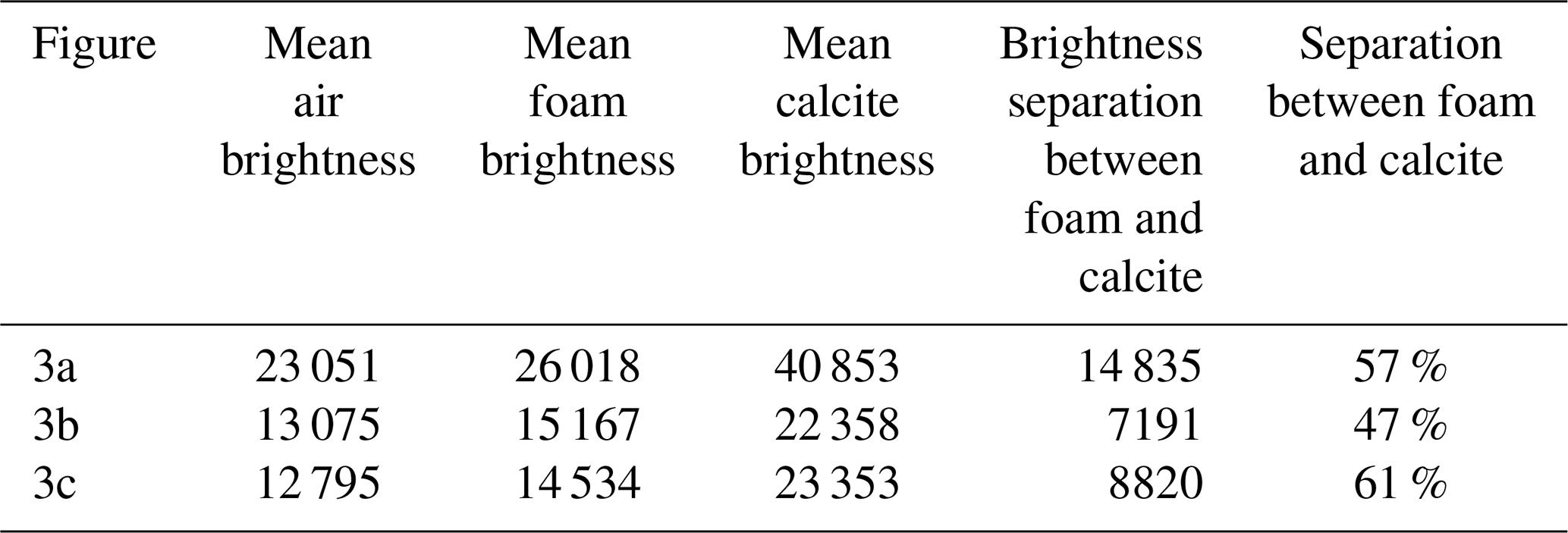
Table 3 Comparison of mean brightness values of air, foam, and calcite (the foraminifer shell) using values from the histograms of Fig. 3a–c.

3.2.6 Scanning time

In a high-throughput setup, both the time taken to set up an automated sequence of tomography points and the scan acquisition time must be considered. Retaining the same scanning parameters for each tomography point minimizes individual specimen setup time, assuming common settings from a suitable compromise for all specimens being scanned. The scan acquisition time is dependent on the beam power, exposure time, number of projections, and detector binning, which all impact the image quality, signal-to-noise ratio, contrast, and resolution. In our case study, with a field of view of 1 mm, we used an X-ray source excitation voltage of 110 kV and a power of 10 W, a 2× spatial binning, and an exposure time of 1.3 s for each of the 1101 projections to achieve a 1 h scan time. The field of view was consistently set for the largest specimen in the set, which we note sacrificed some potential resolution for smaller specimens but was faster to set up and made each scan directly comparable – if it looked bigger, it was bigger.

3.2.7 Specimen reconstruction

Each projection is captured on a detector, and the brightness at each pixel is converted into numbers on a greyscale value between black and white using mathematical transformations and materials of known density for calibration.

Software-based reconstruction filters improve the image quality by reducing streak, bloom, and ring artefacts, along with beam-hardening effects. In our case study, we applied a sharp reconstruction filter with a beam-hardening correction of 1.0 to further reduce beam-hardening artefacts through mathematical transformations.

The centre of rotation of the axial slices (looking down at the sample from the top) is identified algorithmically; once identified, the individual projections are stitched together around the centre of rotation to construct a 3D volume.

As the projection images contained only a single specimen within the surrounding foam, these projections were free from distracting additional regions of higher density, which was optimal for speed and accuracy for the reconstruction algorithms. The resulting reconstructed 3D volume featured a centred specimen with brighter grey values surrounded by darker foam values with sufficient contrast to use a simple brightness thresholding to separate the two. With each volume containing only one specimen and sufficient contrast, we were encouraged to automate the segmentation process and computerized feature identification, resulting in faster throughput of image reconstructions and post-processing analysis of the data because there is no need to separate specimens as unique regions of interest and reduce human-induced uncertainties.

Some reconstruction software allows the application a custom byte-scaling range, which sets the minimum and maximum greyscale values used in the reconstructed scan volume. Byte-scale ranges are bounds to the linear scaling of the original pixel values to fit within the custom range. Selecting a custom byte-scaling range that bounds the specimen's greyscale range results in an image with improved contrast and brightness that enhances the specimen and diminishes speckles from the foam. Unlike dynamic byte-scaling ranges that are derived from the underlying 2D images, which themselves are influenced by the variable instrument parameters and performance, setting custom values provides control for greyscale range consistency within the 3D volume. We consistently applied a byte-scaling range (−0.04 to 0.10) across all our reconstructed .tiff images to make the brightness within each image comparable between scans.

Table 4 Summary of the effects of increasing and decreasing each X-ray CT scanning parameter, as discussed in suggestions 4–8.

4 Output files and post-processing

The reconstructed three-dimensional volume is a numerical representation of the specimen and the surrounding foam and straw. This volume must be saved to a computer file before it can be used outside of the reconstructor software. Various file types are available for saving 3D volume data, with common options including raw data files or uncompressed image stacks, both of which are open and free formats. An image stack comprises a sequence of 2D images visualizing grey values that depict 3D slices in the axial view. Numerous image processing software options facilitate tasks such as noise reduction, contrast adjustment, and filtering, followed by region-of-interest segmentation and volumetric analysis. In line with open-access research principles advocated by Wilkinson et al. (2016), we encourage the use of any suitable file format (such as .tiff or .raw) that aligns with principles of accessibility, interoperability, and reusability for reconstructed micro-CT data.

We chose to export our 3D volume reconstructions as image stacks of .tiff files for wide compatibility with each software package used in our end-to-end methodology and to simplify data sharing with non-micro-CT experts, collaboration between other researchers, and long-term archival of reconstructed CT data. We used ORS Dragonfly (2022) to manually segment regions of interest for bespoke research questions and for labelling individual images to use as inputs for more automated feature extraction as training data in other projects (e.g. Mulqueeney et al., 2024).

The accuracy of threshold-based segmentation from reconstructed .tiff image stacks is influenced by the scanning parameters, which determine contrast, brightness separation, and the presence of artefacts. Higher X-ray energy (e.g. 80 kV) improves material differentiation by increasing the attenuation contrast between calcite and the surrounding medium, resulting in clearer segmentation boundaries. Lower-energy scans (e.g. 40 kV) enhance internal contrast within the foraminifer shell but reduce the separation between foam and calcite, making threshold selection more challenging. Exposure time and detector binning also impact segmentation precision; longer exposures (24 s) and lower binning (2×) produce higher-resolution images with well-defined edges, facilitating more accurate segmentation. In contrast, shorter exposures (15 s) and higher binning (4×) introduce increased noise and reduced boundary sharpness, complicating the differentiation of materials. The number of projections and total scan time further affect reconstruction quality, with 1101 projections reducing streak artefacts and improving segmentation fidelity compared to scans with 701 projections. Figure 3 is a demonstration of how the scanning recommendations presented here can be optimized for achieving reliable threshold-based segmentation of foraminiferal calcite. Reliable segmentation encourages future developments in automatic and programmatic feature extraction from the reconstructed .tiff images for increased automation and reduction in manual processing time.

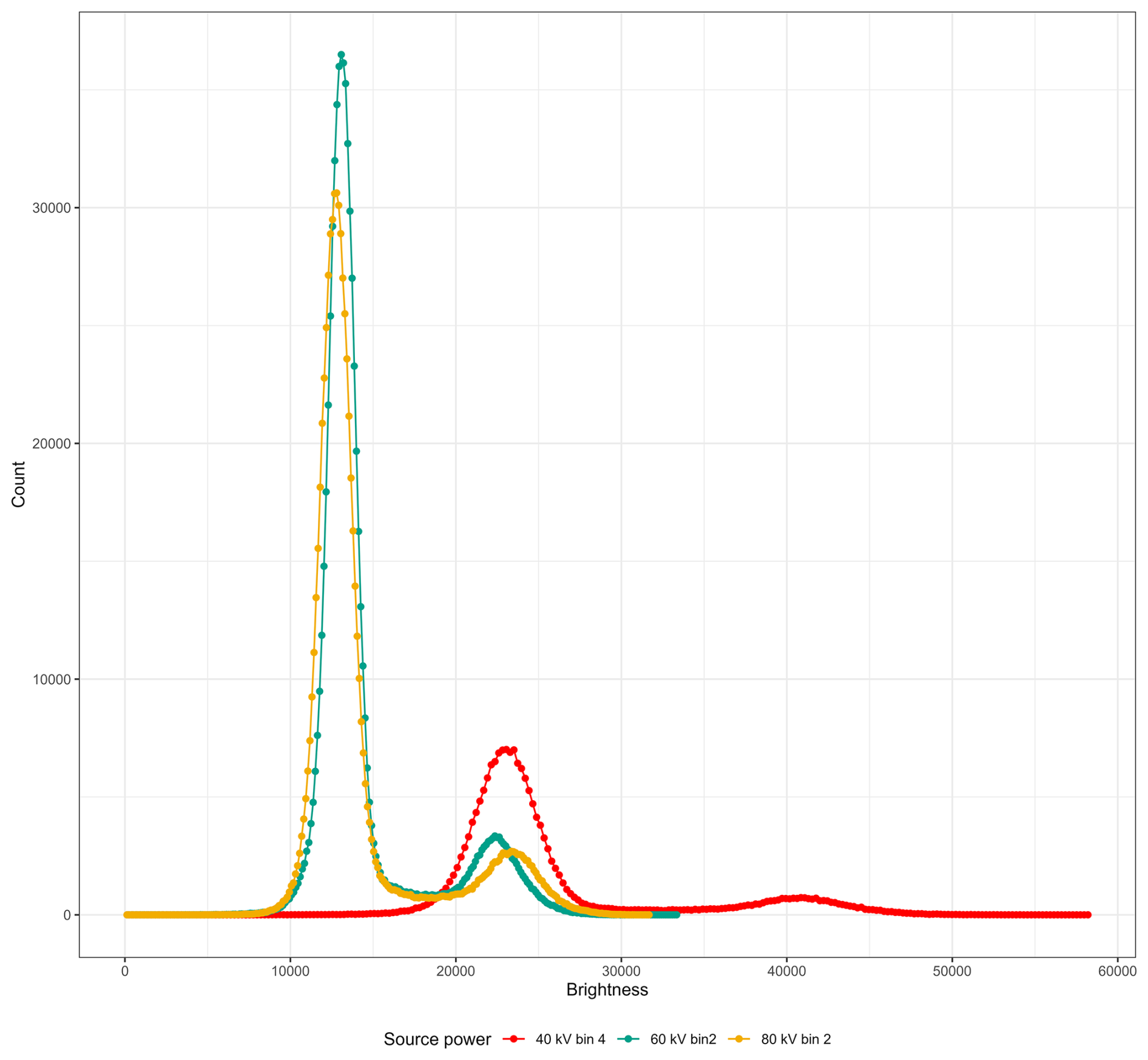
Figure 4 X-ray intensity (counts) by brightness (greyscale) value for the same Dentoglobigerina altispira foraminifer embedded in foam within a plastic straw scanned under varying X-ray source power. Scan parameters are given in Table 2, and each is coloured here as (a) 40 kV source power and detector binned 4× in red, (b) 60 kV source power and detector binned 2× in green, and (c) 80 kV source power and detector binned 2× in yellow.

5 Comparison of scanning parameters

To demonstrate the impact of adjusting the number of radiograph projections (guidelines 2, 3, 4, 6, 8), beam energy and power (5), exposure time (6), and detector binning (7) on the reconstructed 3D image slice, we repeatedly scanned without filtration the same planktonic foraminifer with four parameter permutations. Table 2 lists each scanning parameter, the resulting scan time, and the file size of a single slice from the reconstructed .tiff image stack. All of these slice images are presented in Fig. 3 and have been reconstructed using the same byte-scaling and resized for ease of comparison. The intensity at each brightness (greyscale) value for each of the slice images (Fig. 3a–c) is shown in Fig. 4 and given in Table 3 to illustrate the link between the scanning parameters, the separation between region-of-interest peaks, and the final reconstructed .tiff image.

A lower-power X-ray beam has a lower signal-to-noise ratio because of the reduced photon intensity and can cause photon starvation in extreme cases. This can lead to grainy or noisy images, making it more challenging to discern fine details such as the edges of the surrounding foam. Figure 3a uses a higher binning to improve detector sensitivity and increase exposure. The combination of highest binning and fewest projections produced the fastest scan time and smallest file size. The resulting image shows a visibly sharp boundary between the foraminifer and the surrounding foam, with the widest absolute brightness separation (contrast) between the two materials of the scans presented here.

Using Dragonfly, we identified the lower and upper brightness bounds for the air, foam, and calcite in each scan (Fig. 3 and Table 3). We identified the identity of each of the three peaks in the image histogram using the identified lower and upper bounds then calculated the brightness separation between the foam and the calcite peaks. While all the scans presented here have sufficient brightness separation (contrast) for isolating the foraminifera calcite shell from the surrounding foam and air using threshold segmentation, a wider contrast aids both scientists and computers in feature extraction.

Having kept the magnification, beam filter, and image processing consistent, the calcite brightness is a consequence of altering one or more of the magnification, exposure, projection, energy, and power parameters. In the presented case study, we note that Fig. 3a, with the setup of the fewest projections and the lowest beam energy and power (guideline 5) with the largest detector binning (guideline 7), results in the fastest scan time (guideline 8) and exhibits the widest contrast between foam and calcite (14 835 grey value or 57 % increase). On the other hand, Fig. 3c, with the setup of the highest beam source power (guideline 5) of the study and with more projections (guideline 4), results in an intermediate scan time with a higher spatial resolution and exhibits the widest relative contrast (8820 grey value or 61 % increase).

We highlight the impact that detector binning has on the level of detail captured in the imaging process, with higher binning values generally resulting in a coarser spatial resolution. The spatial resolution for scan A employs a 4× detector binning configuration, leading to a proportionate reduction in resolution to 1370 nm compared to scans B and C, which employ a 2× detector binning setup, achieving a 685 nm resolution.

The interconnected nature of the beam energy and power, detector binning, and exposure time has been presented here in a case study to optimize each parameter for a single foraminifer and is summarized in Table 4. While scanning a single isolated specimen will likely need one set of parameter values, larger studies involving multiple individuals will mean additional considerations should be made regarding total scan time and consistency across specimens. The parameter values needed to obtain a suitable image vary as widely as the range of specimens that can be scanned by micro-CT as a tool to answer research questions – be they environmental, ecological, or evolutionary.