Factors affecting consistency and accuracy in identifying modern macroperforate planktonic foraminifera

Planktonic foraminifera are widely used in biostratigraphic, palaeoceanographic and evolutionary studies, but the strength of many study conclusions could be weakened if taxonomic identifications are not reproducible by different workers. In this study, to assess the relative importance of a range of possible reasons for among-worker disagreement in identification, 100 specimens of 26 species of macroperforate planktonic foraminifera were selected from a core-top site in the subtropical Pacific Ocean. Twenty-three scientists at different career stages – including some with only a few days experience of planktonic foraminifera – were asked to identify each specimen to species level, and to indicate their confidence in each identification. The participants were provided with a species list and had access to additional reference materials. We use generalised linear mixed-effects models to test the relevance of three sets of factors in identification accuracy: participant-level characteristics (including experience), species-level characteristics (including a participant's knowledge of the species) and specimen-level characteristics (size, confidence in identification). The 19 less experienced scientists achieve a median accuracy of 57 %, which rises to 75 % for specimens they are confident in. For the 4 most experienced participants, overall accuracy is 79 %, rising to 93 % when they are confident. To obtain maximum comparability and ease of analysis, everyone used a standard microscope with only 35× magnification, and each specimen was studied in isolation. Consequently, these data provide a lower limit for an estimate of consistency. Importantly, participants could largely predict whether their identifications were correct or incorrect: their own assessments of specimen-level confidence and of their previous knowledge of species concepts were the strongest predictors of accuracy.

1 Introduction

The taxonomy of planktonic foraminifera is the foundation for understanding many geochemical proxy measurements, biostratigraphic analyses and evolutionary studies. Taxonomic disagreements are particularly problematic in studies that combine data from multiple sources (e.g. Kučera et al., 2005a; Rutherford et al., 1999; Siccha and Kučera, 2017) because such studies implicitly assume that the different researchers used the same taxonomic concepts. Experienced participants in the field are often assumed to be accurate and consistent in any taxonomic identification they perform. Incorrect identifications could lead to the propagation of errors through any further analysis (see Al-Sabouni et al., 2018). Disagreements in identifications (or characterisations of a community of individuals) between scientists can come about for a range of reasons: disagreements over the species list to be used for a study, differences in sampling protocols or choices on how to apply the agreed taxonomic concepts. Each of these could produce differences in the list of species described by a study and some are easier to address than others. However, separating out the relative importance of these different factors has rarely been attempted.

One major reason for disagreements in identifications by different scientists depends on the list of species they recognise and the descriptions they are using to describe specimens. For some species, e.g. Orbulina universa (a sphere), their characteristics of the adult form are distinct enough from every other co-occurring planktonic foraminiferal species that it is relatively easy to agree on the taxonomic concept. However, most species are not that distinctive. Changes in taxonomy occur as a result of molecular evidence or of more detailed studies of morphological characteristics. For example, André et al. (2013) used molecular analyses to show that the two commonly identified morphospecies of Trilobatus trilobus and Trilobatus sacculifer are genetically the same species (along with the less used morphospecies of T. quadrilobatus and T. immaturus) although they are often split based on morphological evidence. If they are grouped in a study, that does not necessarily mean the scientist is incapable of telling the two morphotypes apart; rather, they are following a taxonomic concept that sees them as one biological species.

A study using planktonic foraminifera, the El Kef blind test (Lipps, 1997), was explicitly set up to investigate the implications of different species lists and taxonomic concepts on the interpretation of diversity patterns. The taxonomy of the study interval chosen, the Cretaceous–Paleogene boundary, was known to be particularly unstable with no consensus amongst foraminifera workers (e.g. Canudo et al., 1991; Olsson et al., 1999). Four participants from different taxonomic schools produced species lists which showed large differences (mean correlation among participants for taxa identified by at least two workers was 0.478; Keller, 1997). The participants clearly had very different taxonomic concepts, although they inferred relatively similar diversity patterns. To investigate the implications of different taxonomic concepts for accuracy in modern planktonic foraminifera, Al-Sabouni et al. (2018) asked 21 planktonic foraminifera workers to identify sets of 300 specimens. Although they were all told to follow a specific taxonomy they came from a number of different taxonomic schools, leading to differences in their taxonomic concepts. Fewer than one-quarter of specimens had agreement from more than 50 % of participants, and the average agreement of participants' identifications with the consensus was 77 % of specimens when sieving at > 150 µm or 69 % if a >125 µm sieve was used. Consistency tended to be higher within taxonomic schools, suggesting that even with a list of species names there was disagreement on taxonomic concepts in the modern planktonic foraminifera. More generally, consistency between participants in repeatability studies tends to be lower for poorly described taxa (Zachariasse et al., 1978).

When comparing results between studies which intend to characterise the planktonic foraminifer community of a site, it is important to make sure that sampling protocols were identical, as, for example, sieving at different sizes will produce different communities (Al-Sabouni et al., 2007; Weinkauf and Milker, 2018). Additionally, smaller specimens tend to be more challenging to identify. With recent tropical planktonic foraminifera, samples should be sieved at > 125 µm for community analyses; at smaller sieve sizes many juveniles are present, which are not morphologically distinguishable to species level (Zachariasse et al., 1978; Al-Sabouni et al., 2007). However, the recommended sample size for palaeoceanographic transfer functions is > 150 µm (CLIMAP, 1976), as identifying all the smaller species is less relevant. Some of the previous studies of repeatability have not used consistent protocols making the results more challenging to compare. For example, in the El Kef blind test participants were sent sediment samples and asked to prepare them for analysis; they worked at a range of sieve sizes, which is likely to have contributed to the differences in their results (Keller, 1997). In this study the set-up is based on the recommended protocol for community analyses, i.e. sieved at > 125 µm with participants able to manipulate specimens (cf. Al-Sabouni et al., 2018; Keller, 1997), to make the results more widely applicable.

Even with agreement on a species list with its associated taxonomic concepts and a standardised sampling protocol, some disagreements are likely among scientists. Taxonomy is based on types, or typical examples of the morphospecies concept, but assigning specimens to these types is not always easy. If the specimen is poorly preserved, or a juvenile, or has an atypical morphology, then it may not fit any taxonomic type. Additionally, the preservation of the type itself or the quality of images of it can be very variable making some species concepts more open to interpretation. In such cases, how a person chooses to assign the specimen is likely to vary. That variation can be studied in relationship to an individuals' identification over time, or by comparing consistency among a set of foraminiferal workers. To investigate the consistency of identifications of a single researcher over time, Zachariasse et al. (1978) used sets of 200 specimens from a lower Pliocene subtropical sample sieved at > 63 µm. Sixteen species were identified (not untypical for a site in that environment), and counts on the same day had high levels of consistency, with statistical analysis suggesting samples could have been drawn from the same population. After a year, recounts had slightly larger differences, as a result of inconsistent taxonomic concepts for the smaller specimens of a few species. This result is encouraging for consistency, but it does not test the accuracy of those identifications in relation to known taxonomic concepts.

Previous studies on repeatability have mostly conflated the influence of multiple causes of repeatability, combining differences in species lists, sampling protocols or the application of concepts (Bé, 1959; Ginsburg, 1997; Al-Sabouni et al., 2018). They indicate that agreement is greater within taxonomic schools where species concepts are expected to be more similar, but by combining taxonomic disagreement with other factors, it is not clear what level of consistency could be expected when scientists are using an agreed set of taxonomic concepts. In this study, we investigate how the training of a set of taxonomic concepts relates to the accuracy of the identification of specimens. Participants were taught a standard taxonomy and provided with a species list. By modelling a set of factors thought to be important in the accuracy of taxonomic identifications, we aim to identify the relative contributions of scientist-level characteristics (such as their experience), species-level characteristics (such as whether the species had been taught) and specimen-level characteristics (such as its size) on the accuracy of identifications of planktonic foraminifera. We also investigate whether a person's confidence in their identification is reflected in the accuracy.

2 Methods

2.1 Dataset

The specimens in this study were taken from the Ocean Drilling Project (ODP) Site 872 in the west Pacific gyre. Specifically, they were from core 144-872C-1H-1W 80–82 cm which is located at 10.1^∘ S, 162.9^∘ E, and has been dated at 0.14 Ma (Pearson, 1995), so all species are extant. The sample had been washed through a 125 µm sieve and then split, using a microsplitter, to contain roughly 300 specimens. All of the specimens had been provisionally identified to species level (using morphological species concepts), and picked into four-well slides. From this species-level dataset, 100 specimens were chosen from the represented species to provide examples of their range of morphologies and sizes, some typical and some less typical. Between one and seven specimens of each of the species were selected, with most species having three or four specimens. (This variation in the number of specimens of each species precluded participants basing their identifications on the number of specimens of that species they had already identified.) As the sample was taken from one split at one site, only 26 of the 36 extant macroperforate species were represented. Additionally rare species were not always represented by enough specimens to characterise the full range of their morphologies. All specimens were chosen to be complete or nearly complete, so as to have all the defining characteristics required for accurate identification.

This analysis was run as part of a NERC funded advanced training short course on “Taxonomy and Biostratigraphy of Cenozoic Planktonic Foraminifera”, taught at the Natural History Museum, London, in February 2017. This course was aimed at PhD and early-career researchers who wished to acquire or enhance their understanding of the taxonomy of Cenozoic planktonic foraminifera and its applications. The attendees of this course made up the majority of the less experienced participants, whilst the four course conveners who also took part made the more experienced group. Some of these attendees had never worked with planktonic foraminifera before, whilst others already had some experience in their taxonomy. The study focuses on the macroperforate species, which were the main group taught during the course, although a few examples of microperforate and benthic foraminifera were included to assess whether they could be distinguished from macroperforate species. The species list (Supplement Sect. S1) was developed based on Kučera et al. (2005b) and Aze et al. (2011), supplemented with the newly described species in Darling et al. (2006), Aurahs et al. (2011), Weiner et al. (2015) and Spezzaferri et al. (2015).

A set of 25 four-well slides was numbered to receive the specimens. The selected specimens were then placed randomly into these slides (but not stuck down). Random sampling without replacement of a sequence of 1–100 determined the order in which they should be placed. Using randomisation prevented second-guessing of the identifications, and meant that any loss of specimens would not alter the validity of the conclusions. All specimens were then imaged and measured (using Image-Pro Premier), to obtain their mean diameter.

Everyone who undertook the identifications was first asked to fill in a checklist of the extant species that they thought they could identify with confidence (see Sect. S1). They then worked their way through the specimens (in no particular order), assigning a species name and a level of confidence in their identification (confident, y; maybe, m; not confident, n) to each specimen. In this process, the participants were able to manipulate the specimens with a paint brush to observe them from multiple angles (cf. Al-Sabouni et al., 2018). Everyone used the same type of microscope (Leica EZ4, 35× zoom), to remove that factor as a possible source of variation in the results. During identification, reference material was freely available (including Kennett and Srinivasan, 1983; Hemleben et al., 1989; Bolli et al., 1985; Aurahs et al., 2011; Weiner et al., 2015) and the mikrotax website (http://mikrotax.org/pforams/index.html; last access: 6 September 2018), and could be consulted whenever desired; however, participants had a time limit for the task (around 8 hours over the duration of the course, although most did not take that long). After completing the study, the participants filled out a questionnaire to record relevant metadata, including information such as their academic career stage, their study group and their previous training. For the full list of questions, see Sect. S2. In total, 23 people completed the study.

Obtaining a “correct” identification is challenging (Al-Sabouni et al., 2018). In this analysis a definitive identification for each specimen was obtained using only the results of the course conveners (i.e. the more experienced participants). Where there was complete consensus between these participants, identifications were taken as correct. Where there was disagreement, a more powerful microscope (Olympus SZX10, with 63× zoom) was used, and an additional expert (Paul N. Pearson, personal communication, 2017) was called in to arbitrate. A consensus was then reached following discussion.

The results were then compiled for analysis in R v. 3.0.5 (R Core Team, 2015). Where confidence was originally marked as between two levels (e.g. “yes” – “maybe”) it was changed to the lower of the two levels (i.e. “maybe”). In the few cases (3.2 %) where no taxonomic identification was given, the specimen was scored as “UnIDd” with a confidence of “n”. Microperforate and benthic specimens were classified as “nonmacro”. Where the specimen had been lost, it was classified as “lost”, with confidence “NA”.

2.2 Analysis

2.2.1 Consistency

Each identification was scored as correct (if it agreed with the definitive identification) or incorrect. Only the specimens that had been lost were excluded from all the analyses; by the end of the identification process 14 specimens had been lost. Initially the median percentage accuracy was calculated (the median rather than mean was used so it is not biased by the extreme values). The accuracy was then calculated separately for the more experienced and less experienced participants; the former being the course conveners and the latter including the course students. As the confidence of the participant is expected to be correlated with accuracy, we determined the influence of both their species-level confidence and their specimen-level confidence. For the species-level confidence estimates, non-macroperforate specimens were not included as a species-level confidence is not meaningful for these. In this study we used relatively low-powered microscopes, so smaller specimens are likely to have been more challenging to identify accurately; we therefore additionally split accuracy by mean diameter (125–200, 200–400, > 400 µm).

The identification of each specimen by each participant was then used to create a confusion matrix, or error matrix, using the package “caret 6.0–80” (Kuhn, 2016). For each species, this calculates the fraction of cases where that species was identified as each of the different taxonomic names, highlighting which taxonomic concepts are being confused. Inter-rater consistency was estimated using Cohen's (1960) kappa (κ); a kappa of 1 indicates perfect agreement, whereas 0 would indicate no more agreement than expected by chance. A set of additional confusion matrices were also created for investigating the effect of the different levels of experience, the confidence in the identifications and the size of the specimens.

2.2.2 Explanatory variables

To quantify whether a species' morphological uniqueness affects the accuracy with which it is identified, a measure of distinctiveness was calculated for each species. Species were scored for a set of traits (trait data from Aze et al., 2011):

1. Chamber arrangement: angulo-conical, clavate, flat, globorotaliform, globular, planispiral (which includes low trochospiral), spherical;

2. Colour: pink, white;

3. Keel: yes, no;

4. Supplementary apertures: yes, no;

5. Wall texture: cancellate (either irregularly or coarsely), hispid, smooth, cancellate with smooth cortex.

These traits were used to create a dendrogram, from which the ED score (evolutionary distinctiveness: the metric was first applied to phylogenies; Isaac et al., 2007) was calculated; larger values are more unique. For modelling purposes, this score was centred on the mean and scaled by the standard deviation.

In the consistency analysis, the researchers were identified as either more or less experienced. However, this split conflates several different aspects. So for the modelling, researchers' experience was instead quantified in two ways. The number of years a person had been working on planktonic foraminifera was measured as a four-level ordered factor split by quantiles: t<0.1, 0.1≤t<1, 1≤t<4 or t≥4; this coding avoids giving undue weight to the most experienced participants. Experience with these planktonic foraminiferal species is also an ordered factor, with a score between 0 and 2 based on the study systems people were most familiar with as follows: 0 = different time period (not Neogene) and different latitude (not tropical/subtropical) or different group (i.e. not foraminifera); 1 = either same time period or same latitude; 2 = same time period and same latitude.

2.2.3 Mixed-effects models

A generalised linear mixed-effects model was run to investigate the predictors of accuracy. The response variable was whether the specimen was correctly identified; as it is a true/false value, binomial errors were used with a logit link function. Specimens identified as “juvenile” or “nonmacro” were not included in this analysis, unlike the consistency analyses, as many of the species-level explanatory variables do not apply to them. The eight explanatory variables can be grouped into three categories. At the species level, they were distinctiveness of that species, the participant's confidence in identifying that species and whether that species was taught on the course (see Sect. S1). At the scientist level, variables included how long that person had been working with planktonic foraminifera, their experience with a tropical extant community and their gender. The specimen-level variables were the participant's confidence in identification of that specimen and the log of the mean diameter (which was centred on the mean and scaled by the standard deviation before analysis). An interaction between log size (measured as the mean diameter) and the other variables was included in the initial model, as the influence of size is likely to depend on the other parameter values. For example, size may be a less strong predictor of accuracy for more experienced researchers. Participant identity, the definitive species identity and (nested within that) the number of the specimen were initially included as random effects. These were modelled as random effects as they are likely to contribute to the accuracy of the identification, but we are not interested in estimating them from the model (Crawley, 2007).

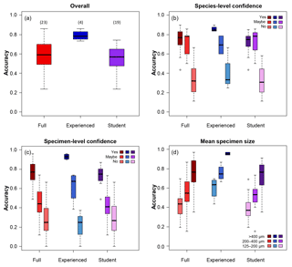
Figure 1 Box plots showing the accuracy of the identifications of the different groups of participants split by different categories. (a) The overall results; numbers in brackets indicate the numbers of participants in each group. (b) Accuracy split by confidence at the species level. (c) Accuracy split by confidence at the specimen level. (d) Accuracy split by the mean size of the specimen.

To determine the optimal random-effects structure, following Zuur et al. (2009), the AIC (Akaike information criterion) value was used to compare all combinations of the random effects fitted to a maximal model. Specimen number nested within species identity was tested with a random slope versus size as well as a random intercept to allow for the possibility that the effect of size on accuracy could be species-specific. Using the optimal random-effects structure and the maximal model, model simplification of the fixed effects was then performed to remove nonsignificant terms (following Crawley, 2007). With the final model, the marginal effects of the variables were determined by removing each explanatory variable in turn from the model and calculating the difference in the R². The analysis was run using “lme4” version 1.1–17 in R (Bates et al., 2015).

Table 1 The percentage accuracy of the different groups of participants, split by species- or specimen-level confidence and size.

3 Results

3.1 Consistency

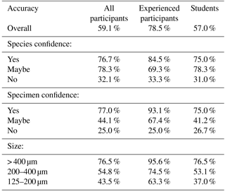
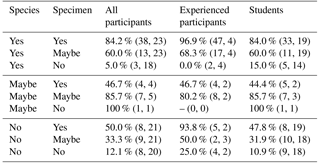
Participants achieved a median percentage accuracy (compared to the definitive ID) of 59 %; the value was 79 % for the four more experienced participants and 57 % for the 19 less experienced participants including students on the course (Table 1, Fig. 1a). When the results are restricted to only include those species the participant is confident in identifying, the median accuracy is 77 % overall (85 % for experienced workers and 75 % for students; Table 1, Fig. 1b). Only 5 of the 26 participants used “maybe” to classify their species-level confidence, so there are few data for that category. Additionally, accuracy was highest (86 %) for the person who was confident in all the species. The percentage accuracy for only those specimens which the participant identified confidently rises to 77 % (93 % for experienced participants, 75 % for students; Table 1, Fig. 1c). Focussing only on those specimens where the participant expressed confidence in both their knowledge of the species and their identification of the specimen, accuracy rises to 84 % overall, and 97 % for experienced participants (Table 2). Larger specimens were more consistently identified correctly (Table 1, Fig. 1d), with accuracy for the largest size fraction (> 400 µm) rising to 96 % for the experienced participants. Everyone had higher accuracy when they were confident (both at species and at specimen levels) than when they were not.

Table 2 The percentage accuracy of the different groups of participants, split by their confidence at both species and specimen level. The numbers in brackets show the median number of specimens (first) for number of participants who used that category (second).

The confusion matrix (Fig. 2) shows the fraction of specimens that were classified under different taxonomic names, with all data included. This matrix had a kappa value of 0.58 which is classified as fair/moderate agreement (Fleiss et al., 2013; Landis and Koch, 1977). Some species, e.g. Pulleniatina obliquiloculata, were identified correctly the majority of the time, whereas others, e.g. Globoconella inflata (which was not taught during the course), were mostly identified incorrectly. For several genera (Globigerinella, Globigerinoides, Globorotalia, Trilobatus), participants mostly identified the correct genus, but were less accurate in identifying the species. For more experienced participants, the kappa value rose to 0.78, considered substantial or excellent agreement; it was 0.54 for students. Kappa was 0.76 for those specimens where people were confident in their identifications, but only 0.21 (indicating poor to slight agreement) for unconfident identifications. For specimens larger than 200 µm, kappa was 0.64 compared with 0.38 for smaller specimens. For the confusion matrices split by participant experience, identification confidence and specimen size see Sect. S3; the numerical versions are available in the data link.

Table 3 The ANOVA for the fixed effects of the final model, showing the degrees of freedom (df), the Chi-squared value (X²) and the p value for each fixed effect.

3.2 Mixed-effects models

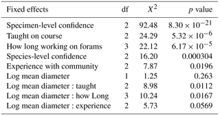
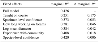
The best random-effects structure, based on AIC, had random slopes versus size for the specimen number nested within species identity and random intercepts for participant identity (see Sect. S4). Following model simplification, the evolutionary distinctiveness and gender terms drop out (for the fixed effects included in the final model and their significance, see Table 3). This model had a marginal R² of 0.43 (the variance explained by the fixed effects) and a conditional R² of 0.57 (variance explained by both fixed and random effects). Of the random effects, most of the variance in the slopes comes from the individual specimens (0.51), whereas the species identity mostly contributed to the intercept (variance = 0.41). The person-level effect did not have random slopes, and had a variance of only 0.11. The results of this model suggest that, irrespective of size, accuracy increases with confidence at both the species and the specimen levels. All the other variables (whether the species had been taught, how long people had worked with planktonic foraminifera and how experienced they were with this community of foraminifera) interacted with log size (Fig. 3). The specimen-level confidence and whether the species was taught were the strongest predictors of agreement (Tables 3, 4).

Table 4 The marginal effects of each explanatory variable. The marginal R² was calculated by excluding that variable (and all its interactions) from the final model. The Δ marginal R² is the difference in the R² from that of the full model.

Size interacts with a set of variables, so its relationship with agreement is more complex. Generally, larger specimens had a higher level of agreement but there are a few exceptions (Fig. 3). Where the species had not been taught on the course, larger specimens were more likely to be identified incorrectly (Fig. 3a). The impact of specimen size is less important for the more practised participants (the relationship levels off at larger sizes, Fig. 3b). Participants with a greater experience of working with the modern planktonic foraminifera tended to be more accurate in their identifications, although the effect is more pronounced at the smaller size fractions (Fig. 3c).

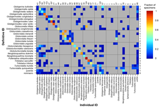
Figure 2 A confusion matrix showing the species that are most frequently confused for all participants. The definitive ID is the taxonomic name considered correct in this study. The individual ID is the name which was given by the participant. For each definitive ID the coloured squares in that row indicate names which were used by the participants for that species. Grey cells indicate that combination did not occur. If all specimens of all species were accurately identified then all the points would plot along the diagonal, with a fraction of 1; additionally each row sums to a fraction of 1. The numbers on the right hand side refer to the number of specimens of that species in the study in the definitive ID. The numbers along the top refer to the number of times that species was identified in the study (n.b. specimens that were lost are excluded from this analysis). κ=0.58. A numerical version of this matrix is to be found in the data link.

4 Discussion

4.1 What affects the accuracy of taxonomic identifications?

Providing accurate identifications of planktonic foraminifera is important for a wide range of subjects, including biostratigraphy, geochemistry and biological research. Our results suggest that, with only a short period of training and relatively low-powered microscopes, researchers are able, on average, to correctly identify 75 % of the specimens belonging to the species they know (Table 1, Fig. 1b). Considering only those specimens of these species for which they express confidence, their accuracy rises to 84 % (Table 2). Accuracy was higher among more experienced participants, for whom the corresponding values are 79 % and 97 %, respectively (Tables 1, 2 and Fig. 1). These results suggest that projects requiring identification of only a few species can be performed well with relatively little training. However, for a complete community analysis of a sample, additional experience and/or more in-depth training are likely to be required.

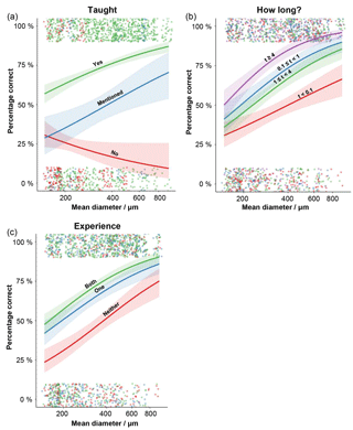
Figure 3 The effects of the interaction terms in the generalised linear mixed-effects model, showing how the size–accuracy relationship is influenced by the different factor levels. (a) The influence of whether the species was taught on the course on the accuracy of the identification. (b) The influence on how long (in t years) the participant had been studying planktonic foraminifera on the accuracy of the identification. (c) The influence of how experienced the participant was on a Holocene tropical assemblage before they started the course; levels record their knowledge of Neogene or tropical assemblages. For each plot, the raw data for each specimen (correct or incorrect) is displayed; points are jittered so they can be seen more clearly. The 95 % confidence intervals around the estimates are also plotted.

By looking further into these results, with a mixed-effects model, we find that the biggest effects on accuracy come from the participants having been taught the species and on the confidence level in the identification of that specimen (Table 4). More generally this indicates that spending time immediately before starting a project refreshing the key characteristics of species that will be the focus of the study is particularly beneficial. Usually, larger specimens have a greater chance of being identified correctly. However, the direction of this trend is reversed in species that were not taught; the largest untaught specimens were likely to be incorrectly identified (Fig. 3a). These results come mainly from two species – Globorotalia theyeri and Globoconella inflata – which are large and were often incorrectly identified. One possible explanation is that participants wrongly assumed all the large species had been taught whereas they were more aware of their lack of knowledge of the smaller specimens. The ED scores, however, dropped out of the modelling, suggesting that species that are similar in general morphology (at least as characterised by these traits) are not consistently confused. This result could indicate that accuracy is more dependent on variation within a species, rather than between species, so it is captured by the species-level random effect. In that case, the inaccurate identifications would mainly result from specimens which are less “typical” examples of a species.

Figure 4 Globoconella inflata (a) and Pulleniatina obliquiloculata (b), scale bar: 200 µm.

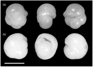
The confusion matrices (Fig. 2, Sect. S3) are particularly useful for identifying the species where people are unsure. These matrices highlight which species are most easily confused; if a participant is focussing on particular species for their study they would obviously do well to consider the distinguishing characteristics from similar species. Often this confusion is within a genus, e.g. the Globigerinella species. For this particular genus there has been a recent taxonomic revision based on molecular work, but supported by the morphology, separating Globigerinella radians from Globigerinella calida (Weiner et al., 2015). Although this distinction was taught on the course it is not included in many of the resources, so there are relatively few images showing the differences, which may partially explain the confusion in that identification. Similarly, recent revisions have occurred in the Globigerinoides genus (Aurahs et al., 2011) reinstating G. elongatus which is likely to have caused similar problems; in this study G. elongatus was often identified as G. ruber. In the case of Globoconella inflata many people were confident that the specimens were Pulleniatina obliquiloculata; these are the only two species in the sample to have a smooth cortex (see Fig. 4), which probably explains the misidentification.

The measures of consistency obtained from this study rely on the “definitive identification” being correct. Without performing DNA analyses (something that would be impossible on this particular set of specimens as they were taken from sediment cores) there is no way of being absolutely certain of the species of a specimen. However, by using the consensus of the more experienced foraminiferal workers (see Sect. 2.1), we have aimed to obtain as “correct” a taxonomy as possible (see Al-Sabouni et al., 2018, for further discussion of this point). This method might tend to cause a slight inflation in the accuracy of the experienced workers, as they are the ones who defined what is correct; however, having an external judge (who was not otherwise involved in the study) for specimens where there was disagreement, should reduce any impact of this effect.

4.2 Other contributing factors

Beyond the variables we were able to model, there are a number of other factors which are likely to contribute to accuracy in the identification of planktonic foraminifera. The power of the microscope being used for the analysis is likely to have a significant effect, particularly at the smaller size fraction. In this study everyone used the same model of microscope to remove any variation from this factor. However, in order to obtain sufficient microscopes for everyone on the course, it was necessary to use relatively low powered (35×) instruments. The sample was sieved at 125 µm, the recommended sieve size for tropical community studies (Al-Sabouni et al., 2007). A size of 125 µm at 35× magnification is equivalent to a size of 180 µm at a more typical 50× magnification. Given the relationship between size and accuracy (observed in this study, and in Al-Sabouni et al., 2018; Zachariasse et al., 1978), it is therefore very likely that with a higher-powered microscope, the accuracy of at least some identifications would increase. Using these rescaled length estimates, the model predicts an increase of approximately 6 % accuracy at 50× compared with 35× magnification, although this effect is more pronounced in the less experienced participants. Therefore, the statistics provided in this study probably represent conservative, minimum estimates of accurate identification.

The mixed-effects models indicate that the largest variation in identification outside the variables we have modelled comes from specimen-level differences. Even after accounting for species identity and size variation within a species, some specimens remain more challenging to identify. The specimens used in this study were chosen to at least have all the defining characteristics, making them easier to identify than more damaged or fragmented specimens. However, they were taken from a typical field sample, so they had a certain amount of sediment still attached making some identifications more challenging. For instance, detecting the presence of supplementary apertures for distinguishing between Globoturborotalita tenella and white morphs of Globoturborotalita rubescens is difficult if the apertures are filled with sediment. Specimens could be cleaned by sonicating them, but that is rarely done to a sample before identification and it is likely to alter the community as thin-walled species are often destroyed (Hodgkinson, 1991). Where accuracy of a particular species is important for a study, then working on clean and whole specimens may be useful.

Species identification was the next most important random effect, whilst person-specific factors (other than experience which was a fixed effect) only had a variance of 0.11. This suggests that the main variation between people occurs as a result of their experience. Gender had no influence on the accuracy of identifications. Additionally, an individual's results can vary over time (Zachariasse et al., 1978). In this study participants were encouraged to focus on accuracy rather than speed in their identifications. Where researchers are working under more time pressure, identifications are likely to be less accurate. Factors such as how tired the participant is, how long they have been identifying samples for that day and whether they are expecting to find a particular species in a sample are also likely to have a small effect on the analysis, but quantifying these additional effects was outside the scope of this study.

The way the specimens were presented might have reduced the accuracy of the identifications. For practical purposes (to enable specimen-level identification), each specimen was placed individually in a slide well. Whilst the presentation we used is more realistic than fixed specimens or images (cf. Al-Sabouni et al., 2018), it is still not completely realistic. More typically, specimens are grouped by species during identification, meaning that morphologically distinct misidentifications are more likely to stand out. Although we were unable to test for the potential positive effects this practice may have, we advise doing so to further reduce the chances of misidentification.

This analysis focussed on one specific time period; however, Zachariasse et al. (1978) pointed out that delimiting species, particularly if multiple samples are compared through time, is challenging with planktonic foraminifera as a result of their very high resolution fossil record. Species descriptions are based on the concept of types, where specimens are related to a typical morphology. When the full ancestor–descendant lineage is present, however, some of the transitional forms will fit more than one morphospecies definition (Pearson, 1998). Our analysis has highlighted that confidence in a species concept tends to increase the accuracy of the identification. However, in a study where that species evolves, confidence in identification might be misplaced.

5 Conclusions and good practice

In this study, we show that one of the largest effects on accuracy was whether scientists were confident in their identification of a specimen. Researcher assessments of their own confidence are largely accurate – they know whether they know – offering a natural path to improved accuracy by re-examining problematic specimens more closely, with more use of literature and/or other people's expertise. Students who have had only a few days of training and who are using low-powered microscopes (35× magnification) are able to accurately identify 57 % of the specimens on average. On the species with which they feel confident, this rises to 75 %. The values for more experienced participants are 79 % and 85 %, respectively. Additionally, participants were generally quite accurately able to judge how confident they were in a specimen's identification, with confident identifications being accurate 75 % of the time (93 % of the time for experienced participants). There was a strong influence of size on the accuracy of the studies, suggesting that on the higher-powered microscopes, more typically used for foraminiferal identification, these percentages could be significantly higher. These results suggest that, even with little training, most participants are able to identify selected species reasonably consistently and that they can identify those specimens where they are unsure and would benefit from additional guidance. However, full community analyses still require more experienced foraminiferal workers.

The median accuracy of 57 % for all the participants found in this study is lower than the 68 % found in Al-Sabouni et al. (2018). These results suggest that, unsurprisingly, it takes more than a few days of training for individuals to become reliable planktonic foraminiferal taxonomists. However, for those species they are confident in, the students were achieving more comparable answers. The more experienced participants here reached a median of 79 %, which is significantly higher than the more global set of participants in Al-Sabouni et al. (2018), suggesting that at least some of the disagreement among workers can come as a result of differences in taxonomic concepts. However, even among experienced participants using the same agreed taxonomy there are disagreements in species definitions.

More generally, there are several things that can be done to minimise taxonomic errors. Taxonomic training is demonstrably beneficial to provide a good grounding in taxonomic concepts. If a study is focussing on particular species (e.g. for isotope analyses), then consider closely related species or those with similar morphology that could be confused. Additionally, picking out clean and whole specimens is likely to give higher accuracy, as well as revisiting specimens where the original identification was unconfident. Before a full community analysis, it is advisable to revisit the taxonomy of the species that are likely to be present to determine how they can be differentiated. Even many of the more experienced workers in this analysis did not know all the species in the recent community, as that is not their main study focus.

Boltovskoy (1965) suggested that the more consistent use of photographs in taxonomic papers would reduce taxonomic problems by making it clearer which species concept is being used. This opinion is still valid today, particularly with the building of large datasets with data from multiple sources, such as the MARGO (Kučera et al., 2005a) and the ForCenS (Siccha and Kučera, 2017) databases. Considering the gradual evolutionary change of many lineages, it is unlikely that taxonomic disagreements will ever be fully resolved. However, if all studies included their taxonomic list and their main references, ideally with associated descriptions or photographs in several relevant orientations, such as is done in Rillo et al. (2016), it would make comparisons between studies more robust.