the Creative Commons Attribution 4.0 License.
the Creative Commons Attribution 4.0 License.
 | 12 Jul 2019
Calcification depth of deep-dwelling planktonic foraminifera from the eastern North Atlantic constrained by stable oxygen isotope ratios of shells from stratified plankton tows
Andreia Rebotim
Antje Helga Luise Voelker
Lukas Jonkers
Joanna J. Waniek
Michael Schulz
Michal Kucera
Stable oxygen isotopes (δ18O) of planktonic foraminifera are one of the most used tools to reconstruct environmental conditions of the water column. Since different species live and calcify at different depths in the water column, the δ18O of sedimentary foraminifera reflects to a large degree the vertical habitat and interspecies δ18O differences and can thus potentially provide information on the vertical structure of the water column. However, to fully unlock the potential of foraminifera as recorders of past surface water properties, it is necessary to understand how and under what conditions the environmental signal is incorporated into the calcite shells of individual species. Deep-dwelling species play a particularly important role in this context since their calcification depth reaches below the surface mixed layer. Here we report δ18O measurements made on four deep-dwelling Globorotalia species collected with stratified plankton tows in the eastern North Atlantic. Size and crust effects on the δ18O signal were evaluated showing that a larger size increases the δ18O of G. inflata and G. hirsuta, and a crust effect is reflected in a higher δ18O signal in G. truncatulinoides. The great majority of the δ18O values can be explained without invoking disequilibrium calcification. When interpreted in this way the data imply depth-integrated calcification with progressive addition of calcite with depth to about 300 m for G. inflata and to about 500 m for G. hirsuta. In G. scitula, despite a strong subsurface maximum in abundance, the vertical δ18O profile is flat and appears dominated by a surface layer signal. In G. truncatulinoides, the δ18O profile follows equilibrium for each depth, implying a constant habitat during growth at each depth layer. The δ18O values are more consistent with the predictions of the Shackleton (1974) palaeotemperature equation, except in G. scitula which shows values more consistent with the Kim and O'Neil (1997) prediction. In all cases, we observe a difference between the level where most of the specimens were present and the depth where most of their shell appears to calcify.
- Article
(2660 KB) - Full-text XML
-
Supplement
(90 KB) - BibTeX
- EndNote


Stable isotope ratios in the shells of fossil planktonic foraminifera have been the backbone of palaeoceanography for more than half a century. This is because during calcification, planktonic foraminifera record the physical and chemical conditions of the surrounding water and the fossil or sedimentary signal can be used to estimate water column properties, such as temperature, salinity or ocean stratification (Emiliani, 1954; Mulitza et al., 1997; Pak and Kennett, 2002; Shackleton, 1974; Simstich et al., 2003; Steph et al., 2009; Williams et al., 1979). The first study using isotope ratios (δ18O) in foraminifera (Emiliani, 1954) revealed species-specific offsets that were attributed to differences in calcification depth among species. This hypothesis was later confirmed by observations from plankton tows (Bé, 1960; Bé and Hamlin, 1967; Berger, 1969; Duplessy et al., 1981; Fairbanks et al., 1980; Lebreiro et al., 2006). Thus, according to their preferred habitat depth, certain species appear to consistently reflect conditions in the surface, whereas others have a more variable calcification habitat and some appear to occur mainly below the mixed layer (Berger, 1969; Fairbanks et al., 1980, 1982; Kemle-von Mücke and Oberhänsli, 1999; Ortiz et al., 1995). Subsequently, it became clear that calcification depth is not a simple reflection of living depth because of factors such as non-linear growth during ontogenetic vertical migration and encrustation (Bemis et al., 1998; Fairbanks et al., 1982; Hemleben et al., 1989; Lohmann, 1995; Mulitza et al., 1997; Simstich et al., 2003). The adult shells, which dominate the >150 µm size fraction of the sediments, reflect an integrated signal of the vertical range where each species lived and calcified (e.g. Birch et al., 2013; Kemle-von Mücke and Oberhänsli, 1999; Steinhardt et al., 2015; Wilke et al., 2009).
In addition, several studies have reported that the isotopic composition of shells of some planktonic foraminifera deviate from the predicted theoretical value for the ambient seawater in which they calcified (e.g. Birch et al., 2013; Fairbanks et al., 1980; Spero and Lea, 1996). The deviation from theoretical values has been attributed to ontogenic or size effects (Bemis et al., 1998; Deuser et al., 1981; Spero and Lea, 1996), symbiont photosynthesis and respiration (Spero and Lea, 1993; Wolf-Gladrow et al., 1999), calcification rate (Ortiz et al., 1996; Peeters et al., 2002), gametogenic or secondary calcite (Bé, 1980; Bouvier-Soumagnac and Duplessy, 1985; Duplessy et al., 1981; Lončarić et al., 2006), and carbonate-ion concentration (Itou et al., 2001; Spero et al., 1997). Size effect due to shell development has been reported in numerous studies with higher δ18O values for larger size fractions (Berger, 1969; Kroon and Darling, 1995; Peeters et al., 2002; Spero and Lea, 1996) and also observed in culture experiments of the species Globigerina bulloides, which when kept under constant temperature and seawater oxygen isotope conditions showed a δ18O increase of up to 0.8 ‰ with increasing size (Spero and Lea, 1996). The addition of a secondary crust in waters deeper (and thus often colder) than the waters of initial shell growth (herein referred to as crust effect), is common in some planktonic foraminifera species (e.g. most globorotalids) during a later stage of their life cycle (Hemleben et al., 1985; Orr, 1967). The secondary crust can contribute up to a third of the total shell mass and therefore skew the result toward a higher δ18O value (Bé, 1980; Bouvier-Soumagnac and Duplessy, 1985; Duplessy et al., 1981; Schweitzer and Lohmann, 1991).
The majority of recent advances in understanding the incorporation of the oxygen isotopic signal are based on the evaluation of signals in foraminiferal shells collected from core-top sediments (e.g. Birch et al., 2013; Cléroux et al., 2007; Durazzi, 1981; Ganssen and Kroon, 2000; Mulitza et al., 1997; Steph et al., 2009). The use of core-top or sedimentary shells to assess how the isotopic signal incorporates in the shell is problematic because the sedimentary signal represents a flux-weighted (seasonal) average of the vertical habitat, integrated over time. A more direct approach is using vertically resolved plankton tows, which allow a direct comparison between the isotopic composition of the shells and the seawater, the vertical abundance distribution of a species and the in situ environmental data (e.g. temperature, salinity) at time of collection. The majority of the studies using plankton tows focused on surface- and intermediate-dwelling species, whereas deep-dwelling species remain poorly constrained (but see Lin et al., 2011; Mulitza et al., 2003; Peeters and Brummer, 2002). This is unfortunate because combining signals from deep dwellers with those from surface- and intermediate-dwelling species is a potentially powerful method to obtain information on the water column structure (Cléroux et al., 2013; Mohtadi et al., 2007; Mulitza et al., 1997; Steph et al., 2009).
Thus, to fully unlock the potential of the geochemical composition of deep-dwelling planktonic foraminifera as a proxy for subsurface conditions, new observations from the water column are needed. Here we present data from stratified plankton tows in the subtropical northeast Atlantic and assess how (or if) the proxy signal preserved in the shells integrates environmental information across the vertical habitat of the foraminifera. We focus on the δ18O signal of the four deep-dwelling species Globorotalia truncatulinoides, G. hirsuta, G. inflata and G. scitula. These species were chosen because they are abundantly present in our samples and occur alive until at least 300 m water depth (Rebotim et al., 2017). We assessed the potential impacts of shell size and secondary calcification, determined if isotopic signal of each species can be predicted by equilibrium calcification considering different palaeotemperature equations, and tested where calcification occurred and if it continued during a presumed ontogenetic vertical migration of the species.
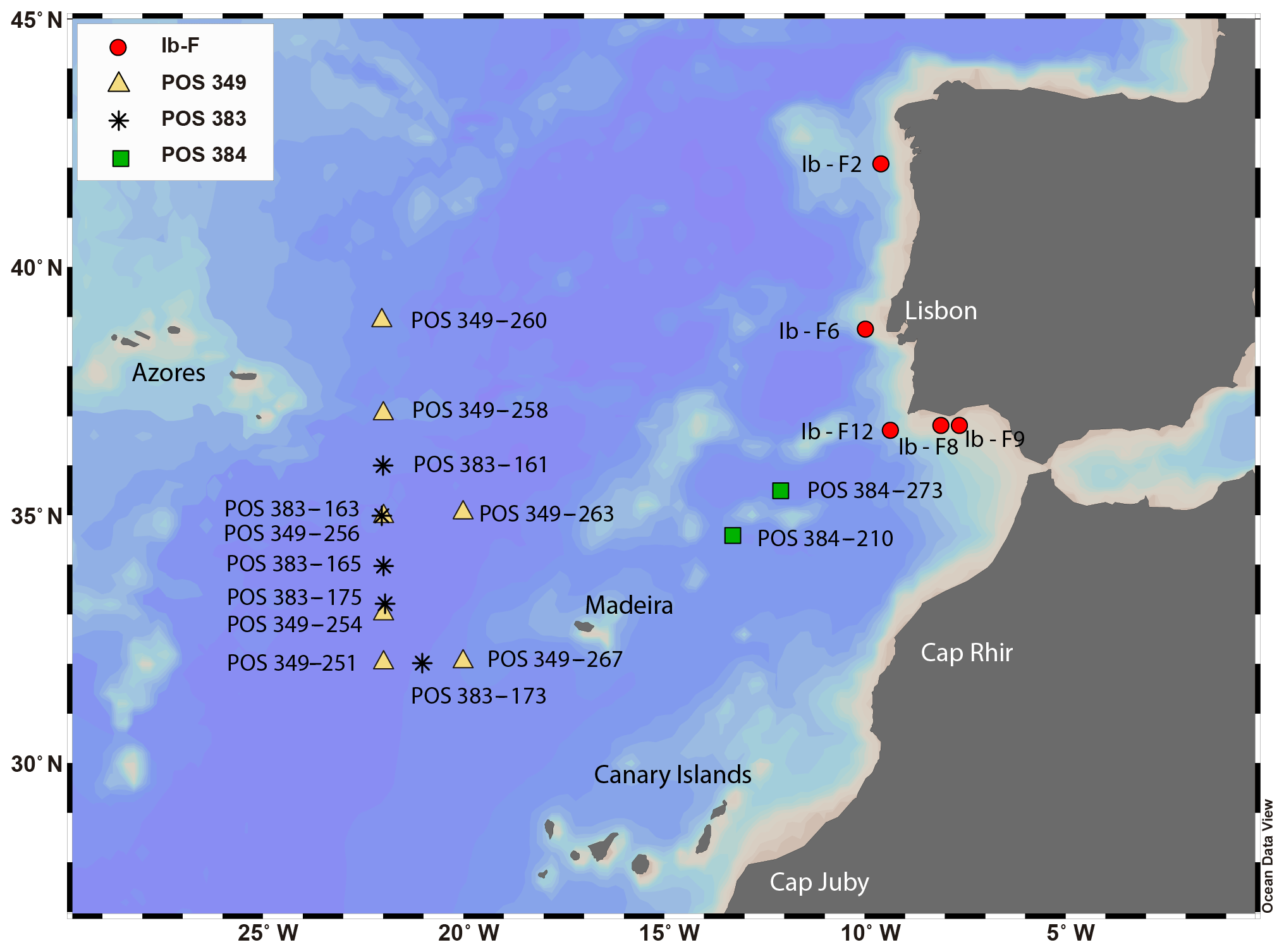
Figure 1Stations in the eastern North Atlantic where planktonic foraminifera for this study were collected from stratified plankton hauls (Table 1). These include 14 stations discussed in Rebotim et al. (2017) and 5 additional stations from the POS 349 campaign. Station symbols are coded by cruise. Map made with ODV (Schlitzer, 2018).
The study area lies between the Azores and the western Iberian Margin, a region influenced by the Azores Current, the Mediterranean Outflow Water and seasonal upwelling (Fig. 1). The Azores Current extends from the southern branch of the Gulf Stream (Sy, 1988) to the Gulf of Cádiz between 32 and 36∘ N (Gould, 1985; Klein and Siedler, 1989), defining the northern limit of the subtropical gyre. Its width varies from 60 to 150 km and its vertical extension can reach 2000 m (Alves et al., 2002; Gould, 1985). The Azores Current is associated with a thermohaline front – the Azores Front, which acts as a border between two different water masses, separating the warmer (∼18 ∘C), saltier and oligotrophic water mass of the Sargasso Sea from the colder, fresher and more productive water mass of the northern and northeastern North Atlantic (Gould, 1985; Storz et al., 2009). This creates an abrupt change in temperature (∼4 ∘C) and in the water column structure across the Azores Front, influencing the distribution of planktonic organisms including foraminifera (Alves et al., 2002; Schiebel et al., 2002). Based on a 42-year-long time series study, the position of the Azores Front varied between 30 and 37.5∘ N (Fründt and Waniek, 2012). Southeast of the Azorean islands, the Azores Current splits into a northern branch that approaches the Portugal Current, a southern branch that connects to the Canary Current and an eastern branch that flows to the Gulf of Cádiz and also along the western Iberian Margin – Iberian Poleward Current (Barton, 2001; Peliz et al., 2005; Sy, 1988). The latter transports eastern North Atlantic Central Water at the subsurface from a subtropical origin (Ríos et al., 1992). The Portugal Current flows southward along the western Iberian Margin, carrying at the subsurface eastern North Atlantic Central Water but of subpolar origin. The North Atlantic Central Water masses form a permanent thermocline that can extend as deep as 800 m (van Aken, 2001). Because of the combination of varied seasonality and the presence of strong gradients in water column structure, the region is particularly suitable to study the calcification behaviour of the deep-dwelling species under variable conditions (Fig. 1, Table 1).
Table 1Cruise and stations, location, time and depth intervals of the collected samples.
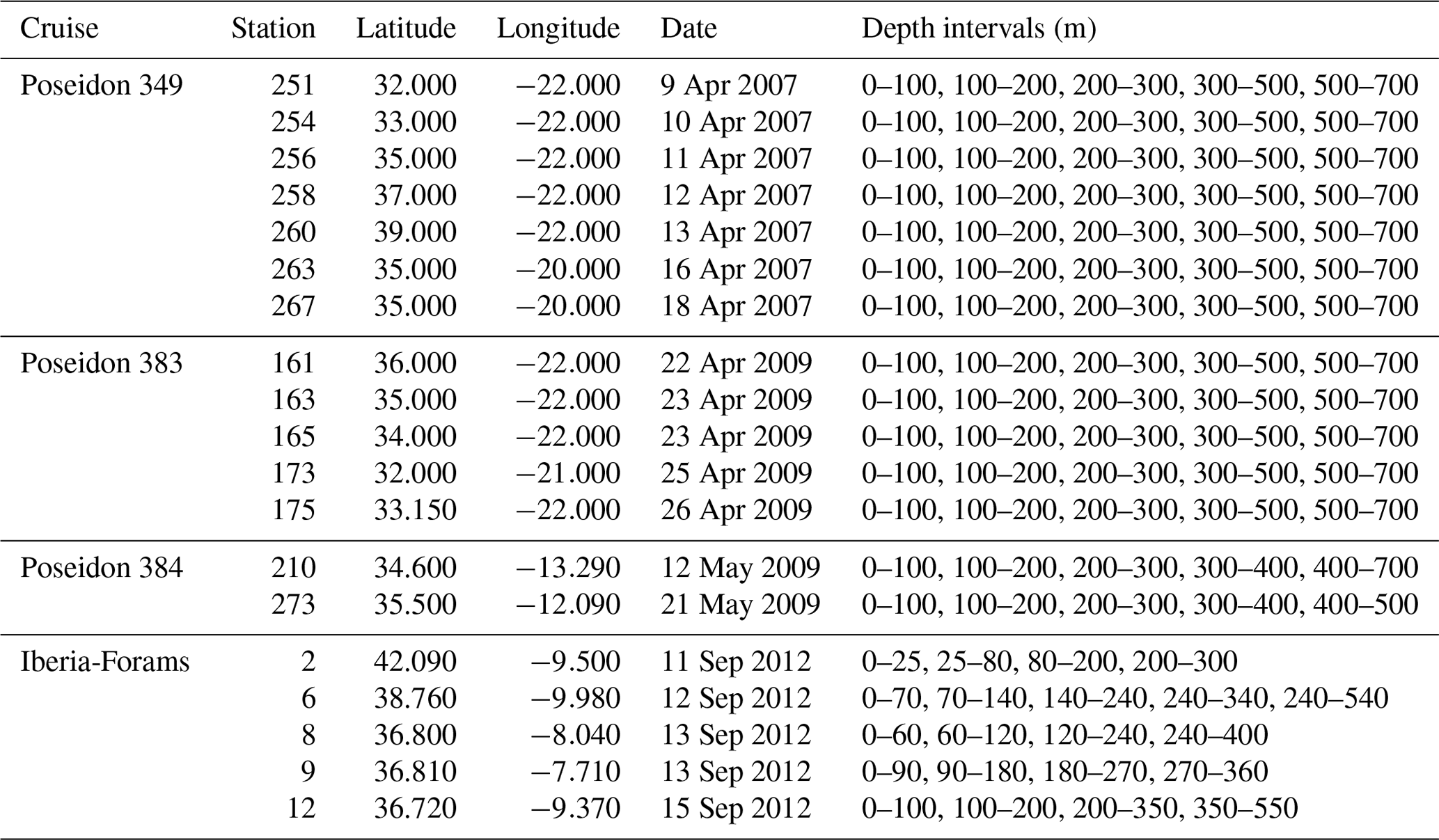
Planktonic foraminifera were sampled during four oceanographic campaigns between 2007 and 2012 in the eastern North Atlantic (Fig. 1, Table 1). The collection was done using Hydro-Bios Midi and Maxi multiple closing nets (100 µm mesh size, opening 50 cm×50 cm) hauled vertically with a velocity of 0.5 ms−1. After collection, the content from each net was transferred to a flask, preserved with 4 % formaldehyde, buffered to a pH value of 8.2 with hexamethylenetetramine (C6H12N4) to prevent dissolution and refrigerated. The abundance of cytoplasm-bearing shells of the four studied species was determined at all stations (Rebotim et al., 2017). In addition, at all stations except two, the abundance of empty shells was used to determine the fraction of the population alive at a given depth interval (see the Supplement for details).
Stable isotope measurements were carried out on cytoplasm-bearing shells picked from two size fractions (150–300 µm and >300 µm; referred to as small- and large-sized fractions, respectively), except for samples of cruise POS 349 where shells were merged across all sizes in the fraction >150 µm. In some cases, especially in G. scitula, it was difficult to distinguish if the cytoplasm was present. In such cases, we used a rule where we considered an opaque white shell empty. For the species G. truncatulinoides only the sinistral variant, which dominated in our samples, was selected for stable isotope analyses. With the exception of the POS 349 samples, specimens with encrusted and non-encrusted shells were separated. In the case of G. truncatulinoides and G. hirsuta this distinction was made by the presence of a thick glassy calcite layer covering the test in comparison with the non-encrusted shells. For G. inflata, the encrusted shells are usually covered by a fine veneer (Hemleben et al., 1985) which has a shiny and smooth appearance in contrast to the non-encrusted individuals. Depending on the species and the size fraction, between 3 and 20 specimens were used for the stable isotope analyses (see the Supplement for details). Whenever possible, replicate measurements were carried out. The samples were not treated prior to analysis.
Stable oxygen isotope measurements, with the exception of POS 349 samples, were performed at MARUM, University of Bremen, using a Finnigan MAT 251 isotope ratio mass spectrometer coupled to a Kiel I or Kiel III automated carbonate device. Isotope ratios are expressed in the δ-notation and calibrated to the Vienna Pee Dee Belemnite (VPDB) scale using the NBS-19 standard. Analytical precision of an in-house carbonate standard (Solnhofen limestone) over the measurement period was ≤0.04 ‰ (1 SD). The POS 349 samples were analysed at the Leibniz Laboratory for Radiometric Dating and Stable Isotope Research, University Kiel, with the Carbo Kiel (Kiel 1) device coupled to a Finnigan MAT 251 mass spectrometer with a precision of ±0.07 ‰ (1 SD) for δ18O for the Solnhofen limestone standard.
Standard deviations among replicates ranged between 0.07 ‰ and 0.11 ‰ among the four species, with an overall mean of 0.08 ‰, which increases to 0.13 ‰ when the full range of the measured values is used, being a more conservative measure considering the low number of replicates per sample. The oxygen isotopic data are provided in the Supplement and will also be stored at the World Data Center PANGAEA (https://www.pangaea.de, last access: 15 May 2019).
To assess if the measured isotopic values could be explained by equilibrium calcification, we calculated oxygen isotope equilibrium values (δ18Oeq) using temperature and salinity data obtained from CTD (conductivity, temperature, depth) casts at the time of sample collection and equations of Shackleton (1974) (Eq. 1) and Kim and O'Neil (1997) (Eq. 2). These palaeotemperature equations were chosen because they are widely used and well established, and cover, due to different calibrations, a reasonable range of possible theoretical δ18O profiles that allows a comparison with our measurements.
where T denotes temperature in degrees Celsius and δ18Ow the δ18O of seawater. For the Shackleton (1974) equation (Eq. 1), the δ18O values from the ambient seawater were converted from VSMOW (Vienna Standard Mean Ocean Water) to VPDB scale by subtracting 0.2 ‰, which was the current conversion at that time (e.g. Pearson, 2012). For the Kim and O'Neil (1997) equation (Eq. 2), the δ18O values were converted from VSMOW to the VPDB scale by subtracting 0.27 ‰ (Hut, 1987). Seawater δ18O was estimated using a regional δ18Ow to salinity relationship (Fig. 2) based on measurements in the study area (24 to 43∘ N and 7 to 34∘ W) (Voelker et al., 2015; and unpublished data for POS 485 from Antje H. L. Voelker), covering the top 700 m of the water column since this is the maximum depth used for the collection of planktonic foraminifera (Eq. 3).
where S denotes in situ salinity at the time of collection. The prediction error calculated for the seawater δ18O estimation was 0.12 ‰. Our regional equation has nearly the same slope (0.55) and intercept (18.98) as the North Atlantic equation of LeGrande and Schmidt (2006). We then compare the oxygen isotope ratios with the vertical distribution of the analysed foraminifera species, as described in Rebotim et al. (2017) and Rebotim (2009) for the POS 349 cruise samples.
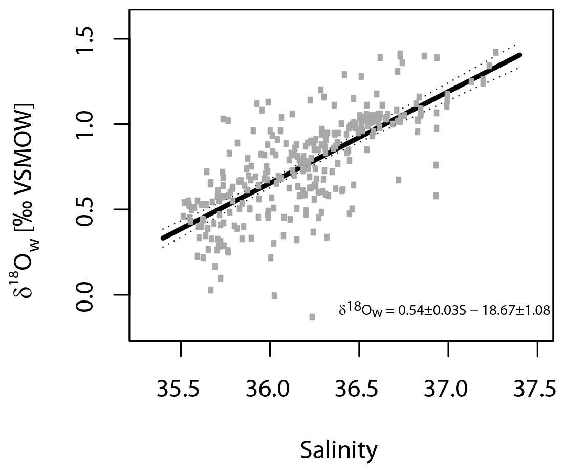
Figure 2Regional linear regression of salinity versus δ18Ow for the eastern North Atlantic Ocean based on data extracted from Voelker et al. (2015) and unpublished data from POS 485. The relationship is based on δ18Ow values (per mil VSMOW) from depths between 0 and 700 m and within the region between 24–43∘ N and 7–34∘ W.
4.1 Vertical distribution of living specimens
At all stations, the vertical distribution of the abundance of cytoplasm-bearing shells indicates that the studied species are found alive across a range of depths, reaching to below the mixed layer (Figs. 3–6). In many cases, the maximum abundance of living specimens occurs below the mixed layer. A broad habitat range is confirmed by the low proportions of empty shells at all but the deepest depth intervals (Figs. 3–6). Among the four species, most of the intercepted specimens (shells) of G. truncatulinoides, G. inflata and G. hirsuta bear cytoplasm down to 500 m, whereas in G. scitula a higher proportion of empty shells is observed already at shallower depths (Fig. 7).
Table 2Size effect between non-encrusted and encrusted specimens and crust effect between specimens with and without crust for the individuals grown under similar conditions, sorted by region.

NA – not available.

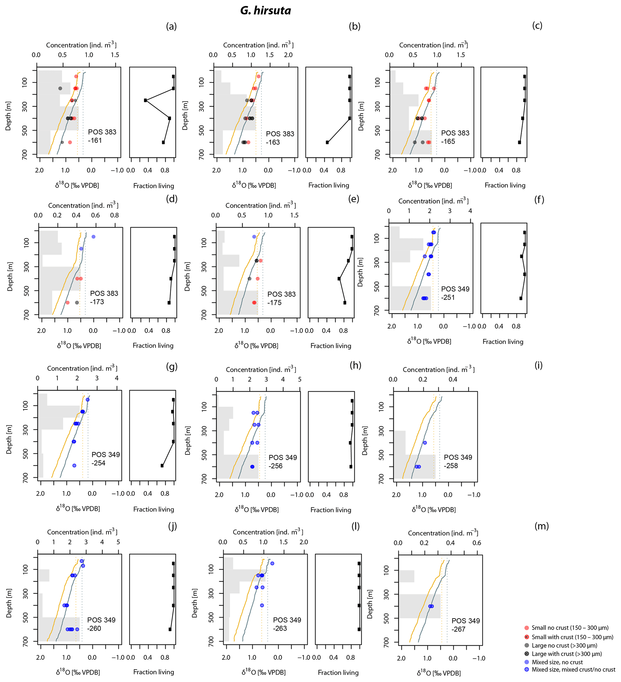
Figure 3Vertical profiles of δ18O, concentration (grey bars, ind. m−3) and fraction of living (cytoplasm-bearing) specimens of the population of G. truncatulinoides in the upper 700 m of the water column at all stations (no data for i and m) with sufficient number of individuals (ind.) for oxygen isotope analysis (Fig. 1). Isotope values are plotted at the mid depth of the collection intervals. Mixed size refers to the size fraction >150 µm. Yellow line shows δ18Oeq for calcite based on the Shackleton (1974) equation; blue line shows the same using the Kim and O'Neil (1997) equation. Dashed lines indicate the mean δ18Oeq values of the upper 100 m. The area between the dashed and solid line for each equation delimit the space of δ18O values that can be explained without requiring disequilibrium calcification.
4.2 Size and crust effects on the δ18O signal of the shell
To assess to what degree the δ18O variability in our data reflects size variation and maturity among the measured specimens, we evaluate the effects of shell size and secondary encrustation (Figs. 3, 4, 5, 6). A potential size effect is observed in non-encrusted G. hirsuta, where δ18O values of larger shells are on average 0.32 ‰ more positive (Table 2). The same appears to be the case for encrusted G. inflata but we refrain from drawing conclusion on this difference as these values are based on two measurement pairs only. The crust effect in this species is almost insignificant for the Iberian Margin sample (0.04 ‰) but it is negative for the sample from the Azores region (−0.12 ‰). Our data do not show a clear indication for a size effect in G. truncatulinoides. However, in this species encrusted small shells have consistently more positive δ18O values than non-encrusted shells (Table 2). The effect of encrustation is unclear for G. inflata and could not be evaluated for G. hirsuta (Table 2). Note that all measurements for G. scitula were made on similar sized specimens, preventing assessment of a size effect.
4.3 Offsets from equilibrium δ18O in the surface layer
Since planktonic foraminifera have been hypothesised to migrate downwards in the water column during growth, a specimen may contain an integrated isotope signature from all depths above the level where it was collected. This integration effect is smallest in the near-surface layer, where migration is likely to be minimal and thermal and isotope gradients are small. Measurements in the surface layer are therefore most suitable to evaluate departures from equilibrium calcification. To this end, we determined the offsets from the two tested equations for the upper 100 m. In this interval, G. inflata and G. truncatulinoides show the smallest offsets from the Shackleton equation, with median offsets of −0.03 ‰ and −0.07 ‰ (Fig. 7). G. hirsuta reveals a difference of −0.11 ‰ from the median value of Shackleton (1974) and 0.11 ‰ from the Kim and O'Neil (1997) δ18Oeq estimate (Fig. 7); thus the δ18O values seem to be equally predicted by both equations. For G. scitula we have only a single measurement in the top layer, showing an offset of −0.06 ‰ from the estimation from Shackleton (1974) and a deviation of 0.18 ‰ from the Kim and O'Neil (1997) prediction (Fig. 7).
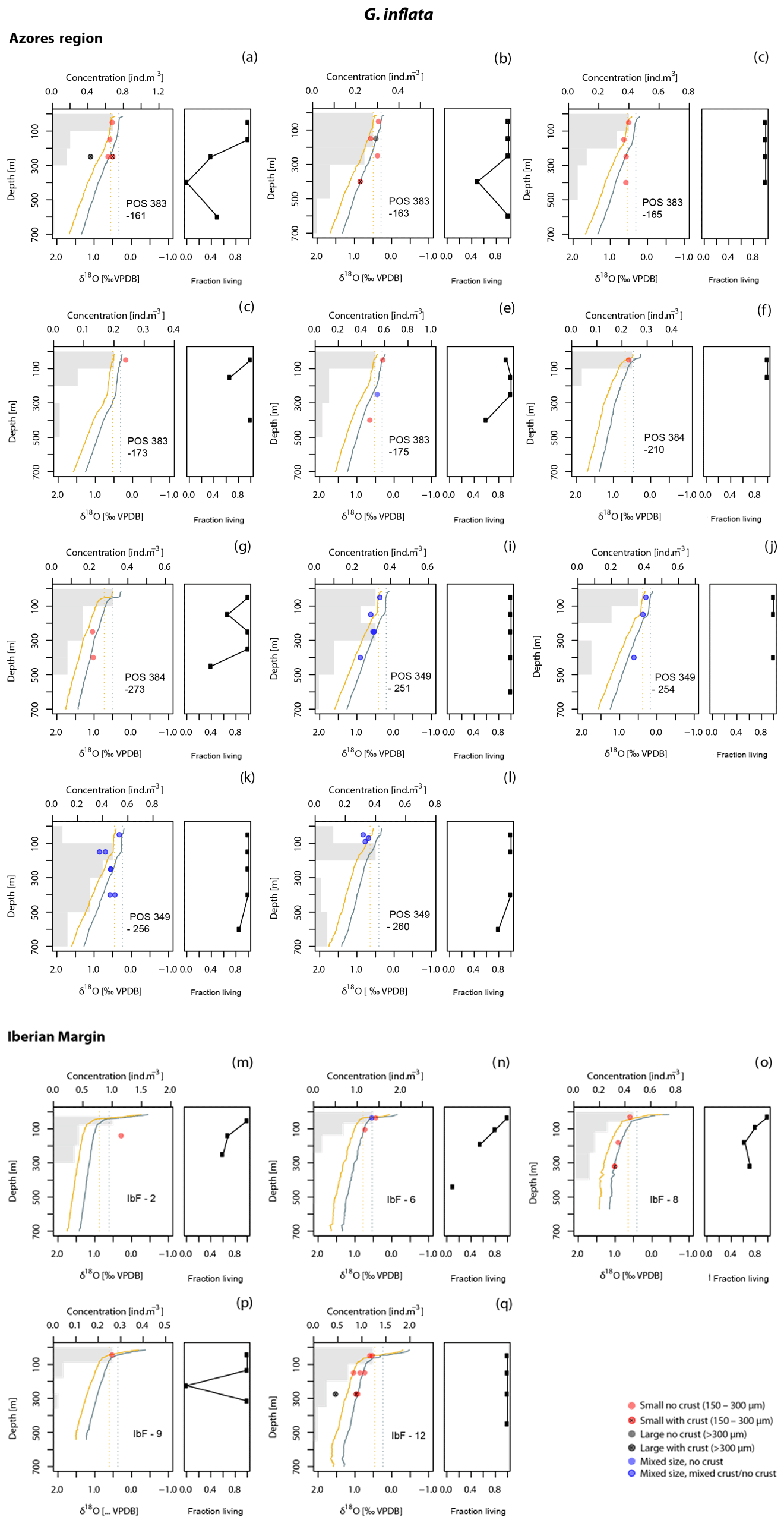
Figure 5As Fig. 3 but for G. inflata, showing separately stations in the Azores Front/Current region and stations along the Iberian Margin. Note that labels (a) to (l) do not correspond to the same stations as in Figs. 3 and 4.
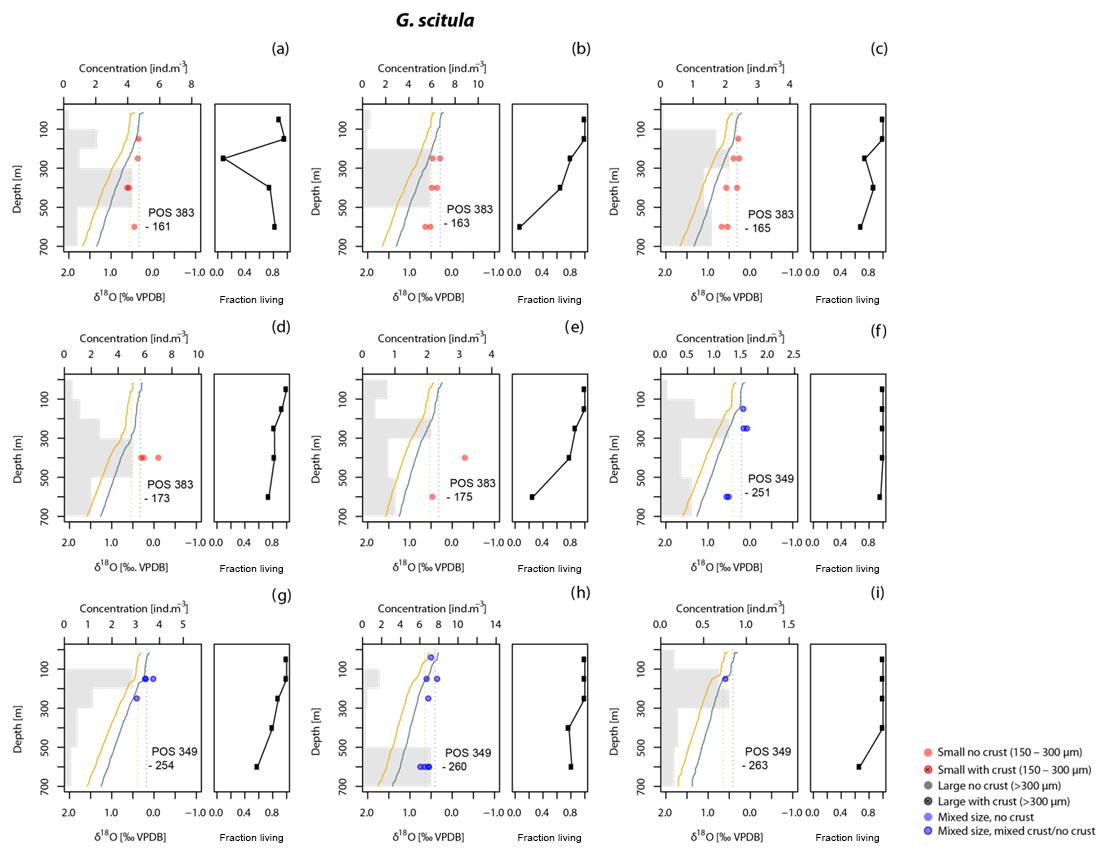
Figure 6As Fig. 3 but for G. scitula. No different size fractions have been distinguished since no specimens >300 µm were found. Stations labelled (a) to (h) are the same as in Figs. 3 and 4.

Figure 7Summary of vertical patterns in foraminifera δ18O and population structure. Left and middle panels show offset from equilibrium δ18O and right panels show average abundance (grey) and the fraction of the population that was collected alive, i.e. cytoplasm bearing. The offsets between foraminifera and equilibrium δ18O are calculated using the Shackleton (1974) and Kim and O'Neil (1997) palaeotemperature equations (left and middle columns, respectively). Solid lines represent the range of δ18Oeq at each depth across all stations. Dashed lines show the range of offsets from the mean near-surface (0–100 m) δ18Oeq values at a given depth. Thick grey line shows the median profile of δ18O offsets for each species. Relative shell concentrations (averaged across all stations where the respective species is present and normalised) are indicated with the grey bar plots in the right column. Note that these serve only to qualitatively assess the vertical abundance pattern and no scale bar is given. Box-and-whisker plots show the range in fraction of living specimens at each depth interval. Each box represents the interquartile range, with the thick black lines indicating the median. The error bars extend to 1.5 times the interquartile range and values outside this range are plotted as dots.
4.4 Vertical patterns in foraminifera δ18O
The δ18O values for G. truncatulinoides become more positive with increasing depth, closely following the δ18Oeq based on the Shackleton (1974) equation down to a depth of 300–500 m (Figs. 3, 7). Below this depth a slight increase in δ18O values is visible until 500–700 m. Similarly, G. hirsuta shows a trend of more positive δ18O values towards deeper waters varying from 300–500 and 500–700 m depth interval, with δ18O values approximating the Shackleton (1974) δ18Oeq line until 300 m (Figs. 4, 7). The highest δ18O values in G. truncatulinoides and G. hirsuta coincide in most of the cases with the presence of a secondary crust or a larger size fraction. G. inflata δ18O values turn slightly positive until approximately 300–500 m (Fig. 5). In comparison, the δ18O values of G. inflata are more positive (0.56 ‰–0.95 ‰) in the stations from the Iberian Margin (Fig. 5) than the δ18O data from the plankton tows from the Azores region (0.19 ‰–0.91 ‰) (Fig. 5), reflecting seasonal temperature differences, namely end of summer for Iberian Margin and spring for Azores. The δ18O values of G. scitula (Fig. 6) remain similar across all depths with δ18O values falling closer to the Kim and O'Neil (1997) estimation than the Shackleton (1974) line (Fig. 7). This species exhibits the lowest δ18O values, between 0.12 and 0.67 ‰.
Before interpreting the results in terms of habitat and calcification depth processes, it is prudent to consider the combined uncertainty in the isotopic values due to non-ecological factors. This combined uncertainty consists of the reproducibility of the measurements (0.13 ‰), the prediction error on seawater composition (0.12 ‰) and the range of isotopic values within the tow intervals. The latter reaches almost 0.5 ‰ and dominates the combined uncertainty, which, assuming that all errors are independent, sums to 0.53 ‰. Thus, in the vertical dimension, only signals exceeding this uncertainty require an ecological explanation. The dominant component of the uncertainty is indicated in Fig. 7, revealing that in all species the observed variability exceeds the uncertainty range. For the interpretation of size and crust effects, only reproducibility (0.13 ‰) needs to be taken into account.
5.1 Size and crust effects in δ18O
To assess to what degree the stable isotopic signatures of the individual species could be interpreted in terms of equilibrium offsets and calcification habitat, we first evaluate the effects of ontogeny on the isotope ratios of the shells. This is essential, because our analysis is based on specimens that were alive during collection and therefore represented different stages in the ontogeny. We focus our comparison on studies of plankton-derived material to avoid the complication of having to consider factors like seasonal integration in the interpretation of size-related trends in sedimentary material (Ezard et al., 2015; Hernández-Almeida et al., 2011). Since few parallel measurements were possible on samples with different shell size or encrustation from the same tow intervals (Figs. 3, 4, 5, 6; Table 2) and the sample sizes are small, our analyses allow the evaluation of shell size and secondary encrustation effects only to a limited extent. The observed trends can, nevertheless, be compared to previous observations on the studied species and to estimate the potential magnitude of the size-related offset and compare it to the magnitude of isotopic variation with depth among the species.
Our observations on non-encrusted G. hirsuta, for which we have most data, show that larger specimens have higher δ18O values, consistent with previous findings (Ganssen, 1983; Hemleben et al., 1985; Niebler et al., 1999). In this species, we also observe that small individuals are present at all depths, but the δ18O values from deeper specimens are consistent with a surface signal, suggesting that these specimens may represent descending individuals that have not yet added any calcite at depth. An increase in the δ18O values with size was also observed for encrusted specimens of G. inflata (+0.58 ‰). Despite the small sample size, the size and amount agree with other authors (Ganssen, 1983; Lončarić et al., 2006; Niebler et al., 1999). In a study performed in the same region, larger specimens of G. truncatulinoides were found to be isotopically higher by 0.4 ‰ (Wilke et al., 2009), which is also in agreement with previous studies in other regions (Hemleben et al., 1989; Lončarić, 2006; Reynolds et al., 2018). The small sample size could potentially explain the apparent absence of a size effect on the δ18O of G. truncatulinoides in our data.
Higher δ18O values in larger specimens could be explained by “vital effects” likely related to calcification rate (Spero and Lea, 1996; Bemis et al., 1998). Alternatively, the same pattern could be explained by ontogenetic vertical migration with a descending trajectory and continued calcification. In this model, the isotopically depleted small specimens at a given depth would represent individuals which calcified at a shallower depth and have not yet added new calcite at the depth where they were collected. Indeed, once these “ontogenetic migrants” add calcite at depth, they also increase in size and are then no longer considered small. These two alternative explanations would leave a different depth-related signature. A “vital effect” would remain constant with depth, whereas ontogenetic vertical migration should cause an increase in the offset between small and large specimens with depth. In our limited data, the observations for G. hirsuta appear consistent with ontogenetic vertical migration, but the data for G. truncatulinoides do not.
Another aspect that affects the δ18O signal is secondary calcification during the final stage of ontogeny (e.g. Bé, 1980; Schweitzer and Lohmann, 1991). Among the studied species, this effect could be observed only in G. truncatulinoides, where encrusted specimens appear isotopically higher by on average 0.27 ‰ (Table 2). For this species, the δ18O increase associated with the addition of a secondary crust has been explored by several authors, who found that the crust may account for 30 % (Mulitza et al., 1997) to more than 50 % (LeGrande, 2004; Lohmann, 1995) of shell mass (e.g. LeGrande, 2004; Lohmann, 1995; Mulitza et al., 1997). For G. inflata, the δ18O difference between non-encrusted and encrusted specimens is not significant or at least inconclusive with the available data (Table 2) and for G. hirsuta the lack of paired data does not allow us to assess this effect.
Typically, isotopically colder signatures in encrusted specimens have been explained by the addition of the crust at the terminal stage (associated with reproduction) or during the final stages of a descending ontogenetic trajectory (Hemleben et al., 1989). If this is true then we should observe encrusted specimens only at depth. Since we observe encrusted specimens at all depths (Figs. 3–6) then either the effects of vertical ontogenetic migration has a limited magnitude or encrustation is not related to the end of the ontogeny. Either way, the higher isotopic values in encrusted specimens could also reflect a different mode of biomineralisation and be the result of a process akin to the size-related vital effect, as also suggested by Kozdon et al. (2009). In addition, studies in trace-metal geochemistry have shown that some planktonic foraminifera species form crusts with different geochemical composition from lamellar calcite grown under the same environmental conditions (Fehrenbacher et al., 2017; Jonkers et al., 2016).
These observations provide first-order constraints for the interpretation of the vertical isotopic profiles. Potential size and crust effects are not seen in all species and their magnitude is <0.5 ‰ (Table 2). Although the size effect could arise either from a vital effect or from ontogenetic vertical migration, the crust effect is more likely a result of a vital effect (different mode or rate of calcification).
5.2 Offsets from equilibrium δ18O in the surface layer
The first-order prerequisite to interpret isotopic signatures in foraminifera is to constrain the presence and magnitude of isotopic disequilibrium (vital effect). Next to culture experiments, material from stratified plankton nets is the only way to directly determine to what degree the foraminiferal calcite was produced in isotopic equilibrium with the surrounding water. The classical ontogenetic vertical migration model with a descending trajectory (Hemleben et al., 1989; Lohmann, 1995) implies that most of the initial calcite shell is built in the surface water, even in deep-dwelling species. To avoid the effect of ontogeny on the observed isotopic values, we here assess the degree of equilibrium calcification only in the surface layer. The equilibrium isotopic composition at each station and depth is constrained by in situ temperature and salinity measurements, but the estimate has to consider differences in palaeotemperature equations commonly used for these (symbiont-free) species of planktonic foraminifera.
In this respect, the δ18O data of G. truncatulinoides show an offset of −0.07 ‰ from the Shackleton (1974) equation (Fig. 7) and a positive offset (0.14 ‰) from the Kim and O'Neil (1997) δ18Oeq prediction (Fig. 7). Lončarić et al. (2006) found in their southeast Atlantic plankton tow samples that above 100 m the δ18O of large specimens (350–450 µm) showed a positive offset (approximately +0.2 ‰) from the Kim and O'Neil (1997) predicted values, whereas the offset was insignificant for small specimens. Ganssen (1983), based on a plankton tow study that applied the Epstein and Mayeda (1953) palaeotemperature equation, which gives values close to Shackleton's (1974), stated that G. truncatulinoides (size fractions: 315–400 µm; 400–500 µm) calcified in equilibrium with the prediction in waters off eastern North Africa. Near the Canary Islands and thus in the vicinity of our study area, δ18O values for smaller (<280 µm) G. truncatulinoides specimens were significantly more negative (−0.22 ‰ to −0.40 ‰) than the predicted δ18Oeq values (Kim and O'Neil equation) within the surface mixed layer (≈120 m) than their larger (280–440 µm) counterparts, whose values were only slightly negative or matched the predicted δ18Oeq values (see Fig. 7 in Wilke et al., 2009).
Similarly, our G. inflata's δ18O values show a negligible negative median offset in relation to the Shackleton estimation (−0.03 ‰) (Fig. 7) and a larger, positive median offset for the Kim and O'Neil line (+0.18 ‰) (Fig. 7). The latter is in good agreement with the Lončarić et al. (2006) observations in the upper 150 m of the southeast Atlantic that showed an offset range between 0.01 ‰ and 0.25 ‰ for the 350–450 µm size fraction relative to the Kim and O'Neil estimation. For the smaller size fraction (200–300 µm) the offset was 0.02 ‰ (Lončarić et al., 2006), which is comparable to the Wilke et al. (2006) findings, who, also using plankton tows from the southeast Atlantic, obtained an average offset in relation to Kim and O'Neil (1997) δ18Oeq of +0.05 ‰ (except for one station) for the size fraction 250–355 µm in the mixed layer. For the samples where size fractions were taken into consideration, the large size fraction is associated with a larger offset, being more positive relative to Kim and O'Neil (1997) δ18Oeq. Using the Epstein and Mayeda (1953) palaeotemperature equation, Ganssen (1983) reports an offset between −0.4 ‰ and +0.5 ‰ for the size fraction 200–400 µm, which is higher than our observed median deviation from the Shackleton's δ18Oeq but smaller than the median offset from Kim and O'Neil's δ18Oeq.
Most of our δ18O data points of G. hirsuta lie closer to the δ18Oeq prediction by Shackleton (1974) (Figs. 4 and 7). For comparison, only plankton tow studies related to the Epstein and Mayeda (1953) δ18Oeq are available. Hemleben et al. (1985) observed a positive offset (0.25 ‰–0.5 ‰) for the large size fraction of G. hirsuta, whereas an offset between −0.5 and +0.2 is reported (200–500 µm) by Ganssen (1983). The only δ18O measurement available for G. scitula in the surface layer falls near the Shackleton prediction, presenting an insignificant offset (Fig. 7). Ortiz et al. (1996), using plankton tows from the northeastern Pacific, estimated a deviation from δ18Oeq (based on Epstein and Mayeda, 1953) of less than −0.4 ‰ for a size fraction >150 µm. Although the offset from Shackleton (1974) δ18Oeq is apparently lower (−0.06 ‰) than that presented by the latter study; it is based on a single measurement and therefore inconclusive.
Thus, in our study, three out of four Globorotalia species show the same trend at the surface, i.e. a small or nonexisting offset from the Shackleton (1974) equation, which may imply that these species have a minimal offset from equilibrium at the surface, except for G. scitula where no conclusion could be made since only a single data point was available. In that species, it is possible that our assumption of using values from the surface layer is incorrect as this species clearly has a subsurface habitat (and abundance maximum) (e.g. Rebotim et al., 2017). At depth, the isotopic values of this species can only be explained by equilibrium calcification when the Kim and O'Neil equation is used (Fig. 7), whereas for the remaining three species the isotopic profiles at depth remain consistent with the Shackleton (1974) equation. The compilation of results from previous studies reveals considerable inconsistencies. These could be real, reflecting unconstrained processes (such as the hypothetical annual reproductive cycle in G. truncatulinoides; e.g. Schiebel and Hemleben, 2017), or they could reflect uncertainties in determining the in situ δ18O of seawater from indirect measurements, which is considerable even in our region (Fig. 2).
5.3 Vertical patterns in foraminifera δ18O: is this evidence for calcification at depth?
In the presence of steep gradients in surface water properties, differences in vertical habitats among species or changes in the vertical habitat of a species during its ontogeny leave a signature in the sedimentary δ18O signal that is at least as important to constrain as the magnitude of disequilibrium calcification. Once the degree of (dis)equilibrium calcification is constrained, the depth interval where calcification occurs can be determined. Although living depth is straightforward to constrain by observations (e.g. Rebotim et al., 2017), the concept of calcification depth requires explanation. Calcification depth could either be considered a specific level in the water column where calcification appears to occur or it can, more realistically as we will explain, refer to the portion of the water column where a species adds calcite to its shell.
Here, we determine the calcification depth assuming that vertical ontogenic migration occurs and that it can be described using a framework of a monotonously descending trajectory and continuous calcification (Hemleben et al., 1989). This hypothetical model can be translated into a concept of vertical changes in isotopic composition, e.g. as implemented by Wilke et al. (2006), in which the δ18O of a foraminifera at a given depth must fall between the surface δ18O equilibrium and the δ18O equilibrium at that depth. Thus, for each vertical profile a theoretical δ18O interval would exist (Fig. 8). The vertical profile of the foraminifera δ18O within this interval describes where the calcite of a specimen from a given depth has been added. If the profile is vertical, all calcite would have to originate from the same depth layer. Such a species would thus theoretically have a preferred calcification depth, which may be different from its living depth. If the vertical profile for a given species follows exactly the predicted δ18O equilibrium profile then all calcite must have been formed at the depth where the specimen was collected. Such a species may have a preferred living depth, but it has no preferred calcification depth. This concept can be verified by considering the vertical profile of the ratio between cytoplasm-bearing shells and empty shells of the study species (Fig. 7). Empty shells should occur in larger numbers only below the depth range where calcification is inferred to take place. This approach is fundamentally different from an attempt to determine (apparent) calcification depth from sediment or sediment-trap samples, which cannot be used to answer the question of whether the calcification occurred during ontogenetic vertical migration. Inferred apparent calcification depth based on such material will always be shallower than the calcification zone identified from specimens from vertically resolved plankton net samples, even if the effect of seasonality can be removed from sediment samples or excluded in sediment trap samples. Isotopic offsets between species sampled in sediment material do not reflect the difference in their calcification depths. Rather, they reflect differences in the zone over which calcification occurred, modulated by the pattern of calcite addition during descent and seasonality.
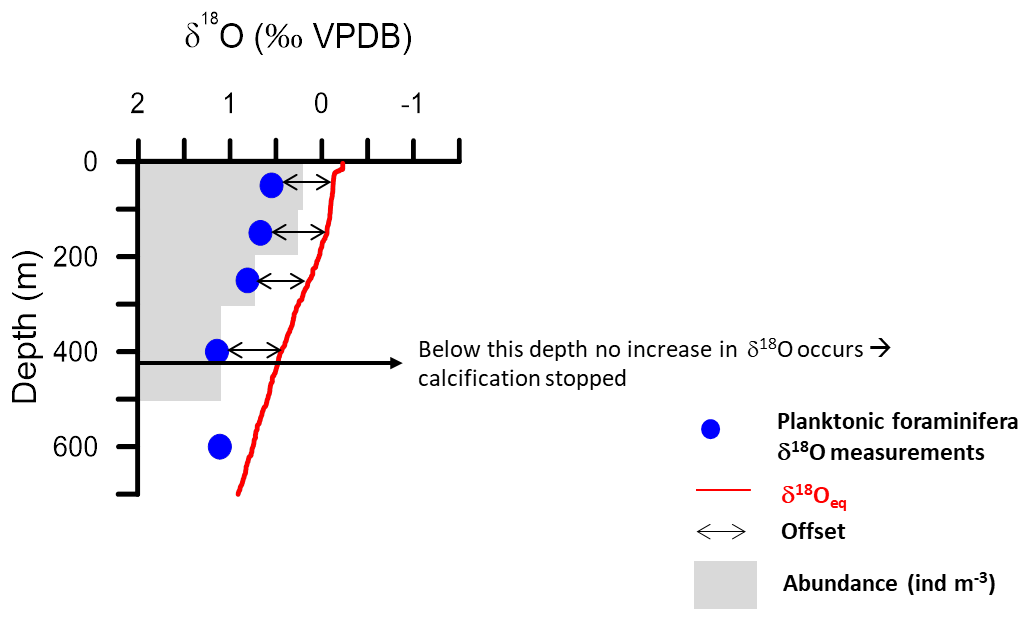
Figure 8Example of an equilibrium calcite δ18O profile based on δ18Oseawater estimated from the regional salinity regression (Fig. 2) and in situ temperature using the Shackleton palaeotemperature equation, compared with δ18O from plankton tow specimens. The diagram is used to illustrate how calcification depth (depth range in the water column where calcification of a given species appears to occur) is defined in this study. The base of calcification depth is defined as the depth below which no increase in δ18O is observed. Offsets of the δ18O values from the δ18Oeq, representing either disequilibrium calcification or vertically integrated calcification, can be quantified within the calcification depth; they are indicated by black arrows.
Following the above framework, the vertical profile of G. truncatulinoides δ18O is consistent with equilibrium calcification following the Shackleton-based prediction from the surface down to 300–500 m (Fig. 7). Below this depth, the isotopic signature remains constant, implying that calcification may cease below this depth. This inference is supported by the increasing number of empty shells below 500 m (Fig. 7). Other plankton tow studies reported that G. truncatulinoides calcified in the upper 200 m in the Sargasso Sea (Hemleben et al., 1985), whereas in the South Atlantic and eastern North Atlantic it was described as calcifying until 400 m (Lončarić et al., 2006; Wilke et al., 2009). Across all stations in this study, the vertical isotopic profile of this species appears to follow the end-member scenario of complete in situ calcification. Remarkably, the observed vertical profile of this species is most consistent with the absence of ontogenetic vertical migration. Despite the obvious variation in living depth captured by our sampling (Fig. 3), specimens outside of the dominant living depth always show an isotopic signature of the depth interval where they were found.
The calcification behaviour inferred from our data implies that a sedimentary isotopic signature of this species should reflect the dominant living depth at a given place. This would provide a new perspective on its variable calcification depth implied by previous studies. Using sediment traps in the Sargasso Sea, Deuser and Ross (1989) and Deuser et al. (1981) estimated that G. truncatulinoides records conditions at 200 m, which is shallower than our observations and could reflect signal integration over a broad depth zone that reaches to the surface. Studies based on surface sediments from the North Atlantic indicate calcification depths between 400 and 700 m (Durazzi, 1981), from 100 to 400 m (Ganssen and Kroon, 2000), and between 200 and 400 m (Cléroux et al., 2007). Other surface sediment studies from the equatorial and South Atlantic estimated calcification depths below 250 m (Niebler et al., 1999), between 270 and 370 m (Steph et al., 2009) or from surface to 700 m (Mulitza et al., 1997). In a modelling approach, Lohmann (1995) estimated a calcification depth between the surface and 800 m and LeGrande (2004) proposed a single calcification depth at 350 m or 30 % of the calcification at the surface and 70 % at 800 m. The diversity of these estimates documents the difficulty to extract information on calcification depth in the absence of knowledge on the actual vertical and/or seasonal abundance of the studied species.
As with G. truncatulinoides, an increase in the δ18O values of G. hirsuta is observed until a depth of 300–500 m (Fig. 4). However, unlike G. truncatulinoides, the vertical isotopic profile of G. hirsuta shows a progressive deviation from the equilibrium at a given depth, consistent with the framework of continued calcification during descent. Below 300 m, the isotopic values in individual profiles appear to stabilise (Fig. 7). This suggests that the calcification depth of G. hirsuta covers the top 300 m of the water column. This would indicate that specimens collected below this depth calcified shallower. Since the abundance maximum of G. hirsuta is below 300 m (Fig. 7), we conclude that the inferred shallower calcification depth is not an artefact of the measurements below 300 m reflecting rare stragglers that may not have yet calcified. In the Sargasso Sea, a plankton tow study also indicated G. hirsuta as calcifying in the first 200 m of the water column (Hemleben et al., 1985). In contrast, in a sediment trap study it reflected average conditions at 600 m (Deuser et al., 1981; Deuser and Ross, 1989) and based on surface sediments it was estimated to have a calcification depth below 250 m in the South Atlantic (Niebler et al., 1999) and between 600 and 750 m in the Atlantic Ocean (Cléroux et al., 2013). Such a large discrepancy could be explained by the addition of a significant amount of secondary calcite below the sampling interval covered in this study (below 700 m), making G. hirsuta a species for which living depth and calcification depth are disconnected.
The vertical isotope profiles of G. inflata are similar to those of G. hirsuta (Fig. 5), consistent with equilibrium calcification and continuous addition of calcite until 200–300 m (Fig. 7). Following the same reasoning as for G. hirsuta, the inferred depth range is unlikely to be an artefact of stragglers. Although the peak abundance of G. inflata is shallower, the population within the calcification depth range is dominated by cytoplasm-bearing specimens (Fig. 7). Using plankton tows from the South Atlantic, this species was reported as calcifying until 400 m (Lončarić et al., 2006), whereas in waters of the NW African upwelling system it is described as calcifying above 200 m (Ganssen, 1983; Wilke et al., 2006). Within the oligotrophic waters of the western Mediterranean Sea a calcification down to 500 m was indicated by van Raden et al. (2011). In contrast, studies based on surface sediments invoke calcification depths between 100 and 250 m in the South Atlantic (Niebler et al., 1999), 100 and 400 m in the eastern North Atlantic (Ganssen and Kroon, 2000), until 400–700 m in the North Atlantic (Durazzi, 1981) and an average calcification of 330–475 m in the Atlantic Ocean (Cléroux et al., 2013). In the case of this species, the overestimated calcification depth in the sediment-based studies likely reflects seasonality. For instance, G. inflata has been reported to reflect winter conditions (Deuser and Ross, 1989; Ganssen, 1983; Wilke et al., 2006; Jonkers and Kucera, 2015), which could be the reason why apparent calcification depth estimations that assume annual calcification are overestimated (significantly deeper).
Contrary to the other species, G. scitula δ18O values appear to be more consistent with the Kim and O'Neil δ18Oeq prediction and its vertical isotopic profiles appears more uniform (Fig. 7). This is consistent with a mode of growth where a large part of the shell calcifies at the top of the interval where the species lives (100–200 m) and very little calcite is added below. Although cytoplasm-bearing specimens dominate at all depth intervals, an increase in the proportion of empty shells in this species occurs shallower than among the other species (Fig. 7). In contrast, Fallet et al. (2011) and Steinhardt et al. (2015), using sediment traps in the Mozambique Channel, postulated that G. scitula calcifies between 200 and 300 m. Greater calcification depths are also invoked in sediment-based studies. Steph et al. (2009) estimated an apparent calcification depth for G. scitula of 300 m in the tropical eastern Atlantic, 200 m in the western Atlantic and below 200 m in the Caribbean. Niebler et al. (1999) proposed a calcification depth below 250 m based on a transect of samples from the South Atlantic. Other factors than those considered in our study (e.g. Itou et al., 2001) may be required to explain the differences in calcification depth derived from our material and other studies but our data clearly show that G. scitula represents an extreme example of a species where living depth and calcification depth differ.
5.4 Contrasting living and calcification depth
We note that for all species at most stations the isotopically inferred calcification depths differ from the observed dominant living depths (Fig. 7). The species G. truncatulinoides shows maximum abundances in the upper 200 m of the water column but calcification occurs in equilibrium until 500 m. Highest abundances for G. hirsuta are observed below 300 m, yet it calcifies throughout the top 500 m. For G. inflata the highest abundances were near the surface but it continues to calcify down to 300 m. Finally, G. scitula is most abundant between 200 and 300 m but its isotopic signal appears to derive from a shallower depth. The different calcification behaviours among the species imply that different aspects of their habitat have to be constrained to interpret their isotopic signatures in sediment samples. Since G. truncatulinoides appears to calcify at all depths, its isotopic signal in the sediment should be the result of integration of populations from different depths. Considering the variation in its depth habitat inferred from plankton tows (Rebotim et al., 2017) and its flux seasonality inferred from sediment traps (Jonkers and Kucera, 2015), the expected sedimentary signal should be weighted towards winter conditions around 100 m water depth. In G. hirsuta and G. inflata, a prediction of the sedimentary signal requires knowledge of the maximum depth at which calcification occurs and a model of how much calcite is added with depth, together with knowledge of the seasonal flux pattern. In G. scitula, the isotopic signature seems to be dominated by conditions at the top of its living depth range, and we observe only a small addition of calcite below 500 m. This is in contrast to the great calcification depth postulated from observed habitat depth and sediment data, unless a significant modification of the isotopic signal occurs below the depth range covered by our study. Nevertheless, it is clear that considering habitat depth alone is unlikely to be sufficient to constrain the depth origin of isotopic signals in planktonic foraminifera.
Using stable oxygen isotope measurements on specimens from stratified plankton net samples, we provide new observations on calcification behaviour of the deep-dwelling planktonic foraminifera species Globorotalia truncatulinoides, G. hirsuta, G. inflata and G. scitula. To assess the potential of these species as a tool to reconstruct subsurface water column properties, we attempt to constrain where in the water column the environmental signal is incorporated in the chemical composition of the shell. We evaluate how the δ18O signal is affected by shell size and the presence of crust, which palaeotemperature equation best predicts the δ18O values of each species and up to what depth the calcification continues.
We show that larger specimens of G. inflata and G. hirsuta appear isotopically higher even when found at the same depth level, which we attribute to ontogenetic migration. A crust effect leading to higher isotopic signal is observed for G. truncatulinoides. This effect likely reflects a different mode or rate of biomineralisation of the crust. These species appear to calcify in equilibrium with the prediction based on the Shackleton (1974) palaeotemperature equation, whereas G. scitula appears better predicted by equilibrium calcification following the Kim and O'Neil (1997) equation.
We infer that G. truncatulinoides does not show a vertical ontogenetic migration and that its sedimentary signal is dominated by the depth and season where it is most abundant (around 100 m in winter). In contrast, G. hirsuta and G. inflata show isotopic profiles consistent with vertical ontogenetic migration and calcite addition until 300–500 m. Interpretation of their sedimentary signals will also require knowledge on the pattern of calcite addition with depth. G. scitula appears to add most of its calcite at the top of the observed living depth range, which seems at odds with its habitat depth and sediment-based calcification depth estimates. In all species we observe differences between living depth and calcification depth, implying that knowledge of both is needed to interpret sedimentary proxy signals of these species.
The data associated with this paper are available in the Supplement and will also be stored at the World Data Center PANGAEA (https://doi.pangaea.de/10.1594/PANGAEA.903668; Rebotim and Voelker, 2019).
The supplement related to this article is available online at: https://doi.org/10.5194/jm-38-113-2019-supplement.
The study was designed by AR, AHLV, LJ, MS and MK. The samples were collected and prepared by AR and JJW. The data analysis and interpretation were carried out by AR, AHLV, LJ and MK. The article was written by AR with feedback from LJ, AHLV, JJW, MS and MK.
The authors declare that they have no conflict of interest.
The master and crew of RV Poseidon and RV Garcia del Cid are gratefully acknowledged for support of the work during the cruises. We would like to thank the chief scientist of the oceanographic campaign Poseidon 384, Bernd Christiansen (Hamburg University) for collecting plankton net samples for us. We thank the editor Kirsty Edgar and Brett Metcalfe and anonymous reviewers for their constructive comments that helped to improve our article.
This research has been supported by the Portuguese
Foundation for Science and Technology (FCT, grant nos. SFRH/BD/78016/2011 and UID/Multi/04326/2019), the European Union Seventh Framework Programme
(FP7/2007-2013) under grant agreement no. 228344-EUROFLEETS and the German Research
Foundation (DFG, grant nos. WA2175/2-1 and WA2175/4-1). Lukas Jonkers received financial support from the German Climate Modelling
consortium PalMod, which is funded by the German Federal Ministry of
Education and Research (BMBF).
The article processing charges for this open-access publication were covered by the University of Bremen.
This paper was edited by Kirsty Edgar and reviewed by Brett Metcalfe and one anonymous referee.
Alves, M., Gaillard, F., Sparrow, M., Knoll, M., and Giraud, S.: Circulation patterns and transport of the Azores Front-Current system, Deep-Sea Res. Pt. II, 49, 3983–4002, https://doi.org/10.1016/S0967-0645(02)00138-8, 2002.
Barton, E. D.: Canary and Portugal currents, Academic Press, 2001, 380–389, https://doi.org/10.1006/rwos.2001.0360, 2001.
Bé, A. W. H.: Ecology of Recent planktonic foraminifera: Part 2, Bathymetric and seasonal distributions in the Sargasso Sea off Bermuda, Micropaleontology, 6, 373–392, 1960.
Bé, A. W. H.: Gametogenic calcification in a spinose planktonic foraminifer, Globigerinoides sacculifer (Brady), Mar. Micropaleontol., 5, 283–310, 1980.
Bé, A. W. H. and Hamlin, W. H.: Ecology of Recent planktonic foraminifera: Part 3: Distribution in the North Atlantic during the Summer of 1962, Micropaleontology, 13, 87–106, 1967.
Bemis, B. E., Spero, H. J., and Lea, W.: Reevaluation of the oxygen isotopic composition of planktonic foraminifera: Experimental results and revised paleotemperature equations, Paleoceanography, 13, 150–160, 1998.
Berger, W. H.: Ecologic patterns of living planktonic Foraminifera, Deep-Sea Res. Oceanogr. Abstr., 16, 1–24, https://doi.org/10.1016/0011-7471(69)90047-3, 1969.
Birch, H., Coxall, H. K., Pearson, P. N., Kroon, D., and O'Regan, M.: Planktonic foraminifera stable isotopes and water column structure: Disentangling ecological signals, Mar. Micropaleontol., 101, 127–145, https://doi.org/10.1016/j.marmicro.2013.02.002, 2013.
Bouvier-Soumagnac, Y. and Duplessy, J.-C.: Carbon and oxygen isotopic composition of planktonic foraminifera from laboratory culture, plankton tows and recent sediment; implications for the reconstruction of paleoclimatic conditions and of the global carbon cycle, J. Foramin. Res., 15, 302–320, 1985.
Cléroux, C., Cortijo, E., Duplessy, J. C., and Zahn, R.: Deep-dwelling foraminifera as thermocline temperature recorders, Geochem. Geophy. Geosy., 8, Q04N11, https://doi.org/10.1029/2006GC001474, 2007.
Cléroux, C., Demenocal, P., Arbuszewski, J., and Linsley, B.: Reconstructing the upper water column thermal structure in the Atlantic Ocean, Paleoceanography, 28, 503–516, https://doi.org/10.1002/palo.20050, 2013.
Deuser, W. G. and Ross, E. H.: Seasonally abundant planktonic foraminifera of the Sargasso Sea: succession, deep-water fluxes, isotopic compositions, and paleoceanographic implications, J. Foramin. Res., 19, 268–293 1989.
Deuser, W. G., Ross, E. H., Hemleben, C., and Spindler, M.: Seasonal changes in species composition, numbers, mass, size, and isotopic composition of planktonic foraminifera settling into the deep Sargasso Sea, Palaeogeogr. Palaeocl., 33, 103–127, 1981.
Duplessy, J. C., Bé, A. W. H., and Blanc, P. L.: Oxygen and carbon isotopic composition and biogeographic distribution of planktonic foraminifera in the Indian Ocean, Palaeogeogr. Palaeocl., 33, 9–46, 1981.
Durazzi, J. T.: Stable-isotope studies of planktonic foraminifera in North Atlantic core tops, Palaeogeogr. Palaeocl., 33, 157–172, 1981.
Emiliani, C.: Depth habitats of some species of pelagic Foraminifera as indicated by oxygen isotope ratios, Am. J. Sci., 252, 149–158, https://doi.org/10.2475/ajs.252.3.149, 1954.
Epstein, S. and Mayeda, T.: Variation of O18 content of waters from natural sources, Geochim. Cosmochim. Ac., 4, 213–224, 1953.
Ezard, T. H. G., Edgar, K. M., and Hull, P. M.: Environmental and biological controls on size-specific δ13C and δ18O in recent planktonic foraminifera, Paleoceanography, 30, 151–173, https://doi.org/10.1002/2014PA002735, 2015.
Fairbanks, R. G., Wiebe, P. H., and Ba, A. W. H.: Vertical distribution and isotopic composition of living planktonic foraminifera in the Western North Atlantic, Science, 207, 61–63, https://doi.org/10.1126/science.207.4426.61, 1980.
Fairbanks, R. G., Sverdlove, M., Free, R., Wiebe, P. H., and Bé, A. W. H.: Vertical distribution and isotopic fractionation of living planktonic foraminifera from the Panama Basin, Nature, 298, 841–844, https://doi.org/10.1073/pnas.0703993104, 1982.
Fallet, U., Ullgren, J. E., Castañeda, I. S., van Aken, H. M., Schouten, S., Ridderinkhof, H., and Brummer, G. J. A.: Contrasting variability in foraminiferal and organic paleotemperature proxies in sedimenting particles of the Mozambique Channel (SW Indian Ocean), Geochim. Cosmochim. Ac., 75, 5834–5848, https://doi.org/10.1016/j.gca.2011.08.009, 2011.
Fehrenbacher, J. S., Russell, A. D., Davis, C. V., Gagnon, A. C., Spero, H. J., Cliff, J. B., Zhu, Z., and Martin, P.: Link between light-triggered Mg-banding and chamber formation in the planktic foraminifera Neogloboquadrina dutertrei, Nat. Commun., 8, 1–10, https://doi.org/10.1038/ncomms15441, 2017.
Fründt, B. and Waniek, J. J.: Impact of the Azores Front Propagation on Deep Ocean Particle Flux, Cent. Eur. J. Geosci., 4, 531–544, 2012.
Ganssen, G. M.: Dokumentation von küstennahmen Auftrieb anhand stabiler Isotope in rezenten Foraminiferen vor Nordwest-Afrika. Meteor Forschungsergebnisse, Deutsche Forschungsgemeinschaft, Reihe C Geologie und Geophysik, Gebrüder Bornträger, Berlin, Stuttgart, C37, 1–46, 1983.
Ganssen, G. M. and Kroon, D.: The isotopic signature of planktonic foraminifera from NE Atlantic surface sediments: implications for the reconstruction of past oceanic conditions, J. Geol. Soc. London., 157, 693–699, https://doi.org/10.1144/jgs.157.3.693, 2000.
Gould, W. J.: Physical oceanography of the Azores front, Prog. Oceanogr., 14, 167–190, https://doi.org/10.1016/0079-6611(85)90010-2, 1985.
Hemleben, C., Spindler, M., Breitinger, I., and Deuser, W. G.: Field and laboratory studies on the ontogeny and ecology of some globorotaliid species from the Sargasso Sea off Bermuda, J. Foramin. Res., 15, 254–272, https://doi.org/10.2113/gsjfr.15.4.254, 1985.
Hemleben, C., Spindler, M., and Anderson, O. R.: Modern Planktonic Foraminifera, Springer-Verlag, New York, available at: http://www.springer.com/gp/book/9781461281504 (last access: 10 December 2015), 1989.
Hernández-Almeida, I., Bárcena, M. A., Flores, J. A., Sierro, F. J., Sanchez-Vidal, A., and Calafat, A.: Microplankton response to environmental conditions in the Alboran Sea (Western Mediterranean): One year sediment trap record, Mar. Micropaleontol., 78, 14–24, https://doi.org/10.1016/j.marmicro.2010.09.005, 2011.
Hut, G.: Stable isotopes reference samples for geochemical and hydrological investigations, Report, Director General. Int. At. Energy Agency, Vienna, 1987.
Itou, M., Ono, T., Oba, T., and Noriki, S.: Isotopic composition and morphology of living Globorotalia scitula: A new proxy of sub-intermediate ocean carbonate chemistry?, Mar. Micropaleontol., 42, 189–210, https://doi.org/10.1016/S0377-8398(01)00015-9, 2001.
Jonkers, L. and Kučera, M.: Global analysis of seasonality in the shell flux of extant planktonic Foraminifera, Biogeosciences, 12, 2207–2226, https://doi.org/10.5194/bg-12-2207-2015, 2015.
Jonkers, L., Buse, B., Brummer, G. J. A., and Hall, I. R.: Chamber formation leads to Mg/Ca banding in the planktonic foraminifer Neogloboquadrina pachyderma, Earth Planet. Sc. Lett., 451, 177–184, https://doi.org/10.1016/j.epsl.2016.07.030, 2016.
Kemle-von Mücke, S. and Oberhänsli, H.: The distribution of living planktic foraminifera in relation to southeast Atlantic oceanography, in: Use of Proxies in Paleoceanography, 91–115, Springer, Heidelberg, Berlin, 1999.
Kim, S.-T. and O'Neil, J. R.: Equilibrium and nonequilibrium oxygen isotope effects in synthetic carbonates, Geochim. Cosmochim. Ac., 61, 3461–3475, https://doi.org/10.1016/S0016-7037(97)00169-5, 1997.
Klein, B. and Siedler, G.: On the Origin of the Azores Current, J. Geophys. Res., 94, 6159–6168, 1989.
Kozdon, R., Ushikubo, T., Kita, N. T., Spicuzza, M., and Valley, J. W.: Intratest oxygen isotope variability in the planktonic foraminifer N. pachyderma: Real vs. apparent vital effects by ion microprobe, Chem. Geol., 258, 327–337, 2009.
Kroon, D. and Darling, K.: Size and upwelling control of the stable isotope composition of Neogloboquadrina dutertrei (d'Orbigny), Globigerinoides ruber (d'Orbigny) and Globigerina bulloides d'Orbigny: examples from the Panama Basin and Arabian Sea, J. Foramin. Res., 25, 39–52, 1995.
Lebreiro, S. M., Frances, G., Abrantes, F. F. G., Diz, P., Bartels-Jonsdottir, H. B., Stroynowski, Z. N., Gil, I. M., Pena, L. D., Rodrigues, T., Jones, P. D., Nombela, M. A., Alejo, I., Briffa, K. R., Harris, I., and Grimalt, J. O.: Climate change and coastal hydrographic response along the Atlantic Iberian margin (Tagus Prodelta and Muros Ria) during the last two millennia, Holocene, 16, 1003–1015, https://doi.org/10.1177/0959683606hl990rp, 2006.
LeGrande, A.: Oxygen isotopic composition of Globorotalia truncatulinoides as a proxy for intermediate depth density, Paleoceanography, 19, PA4025, https://doi.org/10.1029/2004PA001045, 2004.
LeGrande, A. N. and Schmidt, G. A.: Global gridded data set of the oxygen isotopic composition in seawater, Geophys. Res. Lett., 33, L12604, https://doi.org/10.1029/2006GL026011, 2006.
Lin, H. L., Sheu, D. D. D., Yang, Y., Chou, W. C., and Hung, G. W.: Stable isotopes in modern planktonic foraminifera: Sediment trap and plankton tow results from the South China Sea, Mar. Micropaleontol., 79, 15–23, https://doi.org/10.1016/j.marmicro.2010.12.002, 2011.
Lohmann, G. P.: A model for variation in the chemistry of planktonic foraminifera due to secondary calcification and selective dissolution, Paleoceanography, 10, 445–457, https://doi.org/10.1029/95PA00059, 1995.
Lončarić, N.: Planktic foraminiferal content in a mature Agulhas Eddy from the SE Atlantic: Any influence on foraminiferal export fluxes?, Geol. Croat., 59, 41–50, 2006.
Lončarić, N., Peeters, F. J. C., and Brummer, G.-J. A.: Oxygen isotope ecology of recent planktic foraminifera at the central Walvis Ridge (SE Atlantic), Paleoceanography, 21, PA3009, https://doi.org/10.1029/2005PA001207, 2006.
Mohtadi, M., Max, L., Hebbeln, D., Baumgart, A., Krück, N., and Jennerjahn, T.: Modern environmental conditions recorded in surface sediment samples off W and SW Indonesia: Planktonic foraminifera and biogenic compounds analyses, Mar. Micropaleontol., 65, 96–112, https://doi.org/10.1016/j.marmicro.2007.06.004, 2007.
Mulitza, S., Dürkoop, A., Hale, W., Wefer, G., and Niebler, H. S.: Planktonic foraminifera as recorders of past surface-water stratification, Geology, 25, 335–338, https://doi.org/10.1130/0091-7613(1997)025<0335:PFAROP>2.3.CO;2, 1997.
Mulitza, S., Boltovskoy, D., Donner, B., Meggers, H., Paul, A., and Wefer, G.: Temperature: δ18O relationships of planktonic foraminifera collected from surface waters, Palaeogeogr. Palaeocl., 202, 143–152, https://doi.org/10.1016/S0031-0182(03)00633-3, 2003.
Niebler, H.-S., Hubberten, H.-W., and Gersonde, R.: Oxygen isotope values of planktic foraminifera: a tool for the reconstruction of surface water stratification, in Use of Proxies in Paleoceanography, 165–189, Springer, Heidelberg, Berlin, 1999.
Orr, W. N.: Secondary Calcification in the Foraminiferal Genus Globorotalia, Science, 157, 1554–1555, 1967.
Ortiz, J. D., Mix, A. C., and Collier, R. W.: Environmental control of living symbiotic and asymbiotic foraminifera of the California Current, Paleoceanography, 10, 987–1009, https://doi.org/10.1029/95PA02088, 1995.
Ortiz, J. D., Mix, A. C., Rugh, W., Watkins, J. M., and Collier, R. W.: Deep-dwelling planktonic foraminfera of the northeastern Pacific Ocean reveal environmental control of oxygen and carbon isotopic disequilibria, Geochim. Cosmochim. Ac., 60, 4509–4523, 1996.
Pak, D. K. and Kennett, J. P.: A foraminiferal isotopic proxy for upper water mass stratification, J. Foramin. Res., 32, 319–327, 2002.
Pearson, P. N.: Oxygen Isotopes in Foraminifera?: Overview and Historical Review, edited by: Ivany, L. C. and Huber, B. T., Paleontol. Soc. Pap., 18, 1–38, 2012.
Peeters, F. J. C. and Brummer, G.-J. A.: The seasonal and vertical distribution of living planktic foraminifera in the NW Arabian Sea, Geol. Soc. Spec. Publ., 195, 463–497, https://doi.org/10.1144/GSL.SP.2002.195.01.26, 2002.
Peeters, F. J. C., Brummer, G. J. A., and Ganssen, G.: The effect of upwelling on the distribution and stable isotope composition of Globigerina bulloides and Globigerinoides ruber (planktic foraminifera) in modern surface waters of the NW Arabian Sea, Global Planet. Change, 34, 269–291, https://doi.org/10.1016/S0921-8181(02)00120-0, 2002.
Peliz, Á., Dubert, J., Santos, A. M. P., Oliveira, P. B., and Le Cann, B.: Winter upper ocean circulation in the Western Iberian Basin – Fronts, Eddies and Poleward Flows: An overview, Deep-Sea Res. Pt. I, 52, 621–646, https://doi.org/10.1016/j.dsr.2004.11.005, 2005.
Rebotim, A.: Foraminíferos planctónicos como indicadores das massas de água a Norte e a Sul da Frente/ Corrente dos Açores?: Evidências de dados de abundância e isótopos estáveis, Instituto de Ciências Biomédicas Abel Salazar, 2009.
Rebotim, A. and Voelker, A. H. L.: Oxygen isotope data for four deep-dwelling planktonic foraminifera species collected in the subtropical NE Atlantic, PANGAEA, https://doi.org/10.1594/PANGAEA.903668, 2019.
Rebotim, A., Voelker, A. H. L., Jonkers, L., Waniek, J. J., Meggers, H., Schiebel, R., Fraile, I., Schulz, M., and Kucera, M.: Factors controlling the depth habitat of planktonic foraminifera in the subtropical eastern North Atlantic, Biogeosciences, 14, 827–859, https://doi.org/10.5194/bg-14-827-2017, 2017.
Reynolds, C. E., Richey, J. N., Fehrenbacher, J. S., Rosenheim, B. E., and Spero, H. J.: Environmental controls on the geochemistry of Globorotalia truncatulinoides in the Gulf of Mexico?: Implications for paleoceanographic reconstructions, Mar. Micropaleontol., 142, 92–104, https://doi.org/10.1016/j.marmicro.2018.05.006, 2018.
Ríos, A. F., Pérez, F. F., and Fraga, F.: Water masses in the upper and middle North Atlantic Ocean east of the Azores, Deep-Sea Res. Pt. A, 39, 645–658, 1992.
Schiebel, R. and Hemleben, C.: Planktic foraminifers in the modern ocean, Springer, Berlin, Heidelberg, 2017.
Schiebel, R., Waniek, J., Zeltner, A., and Alves, M.: Impact of the Azores Front on the distribution of planktic foraminifers, shelled gastropods, and coccolithophorids, Deep-Sea Res. Pt. II, 49, 4035–4050, 2002.
Schlitzer, R.: Ocean Data View, available at: https://odv.awi.de (last access: 8 July 2019), 2018.
Schweitzer, P. N. and Lohmann, G. P.: Ontogeny and habitat of modern menardii form planktonic foraminifera, J. Foramin. Res., 21, 332–346, 1991.
Shackleton, N. J.: Attainment of isotopic equilibrium between ocean water and the benthonic foraminifera geuns Uvigerina: Isotopic changes in the ocean during the last glacial, Colloq. Int. du C.N.R.S., 219, 203–210, 1974.
Simstich, J., Sarnthein, M., and Erlenkeuser, H.: Paired δ18O signals of Neogloboquadrina pachyderma (s) and Turborotalita quinqueloba show thermal stratification structure in Nordic Seas, Mar. Micropaleontol., 48, 107–125, https://doi.org/10.1016/S0377-8398(02)00165-2, 2003.
Spero, H. J. and Lea, D. W.: Intraspecific stable isotope variability in the planktic foraminifera Globigerinoides sacculifer: Results from laboratory experiments, Mar. Micropaleontol., 22, 221–234, https://doi.org/10.1016/0377-8398(93)90045-Y, 1993.
Spero, H. J. and Lea, D. W.: Experimental determination of stable isotope variability in Globigerina bulloides: Implications for paleoceanographic reconstructions, Mar. Micropaleontol., 28, 231–246, https://doi.org/10.1016/0377-8398(96)00003-5, 1996.
Spero, H. J., Bijma, J., Lea, D. W., and Bemis, B. E.: Effect of seawater carbonate concentration on foraminiferal carbon and oxygen isotopes, Nature, 390, 497–500, 1997.
Steinhardt, J., Cléroux, C., de Nooijer, L. J., Brummer, G.-J., Zahn, R., Ganssen, G., and Reichart, G.-J.: Reconciling single-chamber Mg∕Ca with whole-shell δ18O in surface to deep-dwelling planktonic foraminifera from the Mozambique Channel, Biogeosciences, 12, 2411–2429, https://doi.org/10.5194/bg-12-2411-2015, 2015.
Steph, S., Regenberg, M., Tiedemann, R., Mulitza, S., and Nürnberg, D.: Stable isotopes of planktonic foraminifera from tropical Atlantic/Caribbean core-tops: Implications for reconstructing upper ocean stratification, Mar. Micropaleontol., 71, 1–19, https://doi.org/10.1016/j.marmicro.2008.12.004, 2009.
Storz, D., Schulz, H., and Waniek, J.: Seasonal and interannual variability of the planktic foraminiferal flux in the vicinity of the Azores Current, Deep-Sea Res. Pt. I, 56, 107–124, https://doi.org/10.1016/j.dsr.2008.08.009, 2009.
Sy, A.: Investigation of large-scale circulation patterns in the central North Atlantic: the North Atlantic current, the Azores current, and the Mediterranean Water plume in the area of the Mid-Atlantic Ridge, Deep-Sea Res. Pt. A, 35, 383–413, https://doi.org/10.1016/0198-0149(88)90017-9, 1988.
van Aken, H. M.: The hydrography of the mid-latitude northeast Atlantic Ocean – Part III: The subducted thermocline water mass, Deep-Sea Res. Pt. I, 48, 237–267, 2001.
van Raden, J. U., Groeneveld, J., Raitzsch, M., and Kucera, M.: Mg∕Ca in the planktonic foraminifera Globorotalia inflata and Globigerinoides bulloides from Western Mediterranean plankton tow and core top samples, Mar. Micropaleontol., 78, 101–112, https://doi.org/10.1016/j.marmicro.2010.11.002, 2011.
Voelker, A. H. L., Colman, A., Olack, G., Waniek, J. J., and Hodell, D.: Oxygen and hydrogen isotope signatures of Northeast Atlantic water masses, Deep-Sea Res. Pt. II, 116, 89–106, https://doi.org/10.1016/j.dsr2.2014.11.006, 2015.
Wilke, I., Bickert, T., and Peeters, F. J. C.: The influence of seawater carbonate ion concentration [] on the stable carbon isotope composition of the planktic foraminifera species Globorotalia inflata, Mar. Micropaleontol., 58, 243–258, https://doi.org/10.1016/j.marmicro.2005.11.005, 2006.
Wilke, I., Meggers, H., and Bickert, T.: Depth habitats and seasonal distributions of recent planktic foraminifers in the Canary Islands region (29∘ N) based on oxygen isotopes, Deep-Sea Res. Pt. I, 56, 89–106, https://doi.org/10.1016/j.dsr.2008.08.001, 2009.
Williams, D. F., Bé, A. W. H., and Fairbanks, R. G.: Seasonal oxygen isotopic variations in living planktonic foraminifera off Bermuda, Science, 206, 447–449, 1979.
Wolf-Gladrow, D. A., Bijma, J., and Zeebe, R. E.: Model simulation of the carbonate chemistry in the microenviroment of symbiont bearing forminifera, Mar. Chem., 64, 181–198, 1999.