Identification of living (Rose Bengal)-stained benthic foraminifera using automated image recognition

Living and fossil benthic foraminifera are widely used as bioindicators of ecosystem quality, but their analysis is time-consuming. With the help of artificial intelligence, models for the automatic identification of fossil planktonic foraminifera and, more recently, benthic foraminifera are emerging. Although large datasets of images can now be acquired automatically, efficient processing pipelines are still needed. Here we use convolutional neural networks (CNNs) to automatically identify living benthic foraminifera at the species level. Rose Bengal staining is widely used in ecological and biomonitoring studies to identify living foraminifera, which reflect present environmental conditions. We investigate both low-diversity assemblages from an intertidal mudflat on the French Atlantic coast (Bourgneuf Bay) and high-diversity assemblages from the French Mediterranean coast. Samples were imaged using a modified 3D printer equipped with a camera. The three trained CNN models are efficient in identifying species of the total community (i.e., living and dead foraminifera together) in both low- and high-diversity settings with an accuracy of 96.0 % and 82.2 %, respectively. The results compare well to published indices for ecosystem quality in high-diversity ecosystems. One CNN model can distinguish both species and vital status (i.e., living and dead specimens) for the low-diversity spot with an accuracy of 94.2 %. The results of this first application of machine learning for identifying living benthic foraminifera are very encouraging for improving the efficiency and applicability of these bio-indicators in biomonitoring studies. This approach highlights the potential of automated image-based identification to accelerate the use of benthic foraminifera as bioindicators in large-scale environmental monitoring programs.

1 Introduction

Benthic foraminifera are widely used as bioindicators in biomonitoring studies to assess ecosystem quality in coastal environments (Barras et al., 2014; Dubois et al., 2021; Jorissen et al., 2018; O'Brien et al., 2021; Schönfeld et al., 2012). Their potential for biomonitoring studies arises from their species-specific and rapid response to changing environmental conditions (Gooday et al., 2000; Jorissen et al., 1995, 2018; Murray, 1989, 2006). Furthermore, their small size and high abundance allow for the collection of statistically significant numbers of specimens from minimal sediment quantities, enabling minimally invasive sampling (Barras et al., 2014; Jorissen et al., 2018; Murray, 2006).

In long-term studies, numerous samples have to be analyzed in a limited amount of time to monitor the effect of pollution or climate change. Seasonal variations in population dynamics require high-temporal-resolution sampling and efficiency in data processing. Yet, established protocols require that entire samples are examined for the presence of living foraminifera, which have to be picked and identified manually (including replicate samples). Moreover, it is essential to distinguish living from dead fauna, which is commonly achieved by Rose Bengal staining of living specimens. Further ecological indices utilizing living foraminifera fauna are derived using precisely identified specimens at the species level (Barras et al., 2014; Jorissen et al., 2018).

Foraminifera tests show a variety of morphological features – such as texture, chamber organization, and porosity – that allow them to be identified (Hayward et al., 2020; Jones and Brady, 1994; Jorissen et al., 2023; Loeblich and Tappan, 2015; Milker and Schmiedl, 2012). A total of 9600 modern and 54 600 fossil species have been described today (Hayward et al., 2020). The classical approach for foraminifera identification is to visually inspect each specimen under a stereomicroscope and pick foraminifera individuals one by one, which is time-consuming and requires expert knowledge (Ranaweera et al., 2009). Recently, several studies have shown that the identification of planktonic foraminifera by scientists with different levels of expertise/experience may lead to inconsistencies (Al-Sabouni et al., 2018; Fenton et al., 2018).

With the rise of artificial intelligence, it is now possible to identify different groups of microorganisms, such as diatoms (Bueno et al., 2017; Godbillot et al., 2024; Kloster et al., 2020; Lambert and Green, 2020; Pedraza et al., 2017; Urbánková et al., 2016), coccolithophores (Beaufort and Dollfus, 2004), pollen (Bourel et al., 2020), radiolarians (Keçeli et al., 2017; Tetard et al., 2020), monothalamid foraminifera (Sabbatini et al., 2025), and planktonic foraminifera (Carvalho et al., 2020; Harbowo and Muliawati, 2024; Hsiang et al., 2019; Marchant et al., 2020; Mitra et al., 2019; Piva et al., 2024). Studies taking advantage of artificial intelligence techniques for the automatic identification of benthic foraminifera are rare and focused on fossil faunas from carbonate rock samples (Carvalho et al., 2020), open-ocean cores (Hayat et al., 2026; Johansen et al., 2021; Marchant et al., 2020; Yayan et al., 2024), or fjords (Plavetić et al., 2025). Fossil specimens were automatically classified using convolutional neural networks (CNNs), a well-proven machine learning (ML) technique (He et al., 2015; LeCun et al., 1989). Yet, to the best of our knowledge, these techniques have not been applied to the identification of benthic foraminifera from coastal sediments. Moreover, the differentiation between living (Rose Bengal (RB)-stained) and dead specimens is necessary for biomonitoring purposes, and the problem of color differences within one single species has not yet been tackled. Historical time series of benthic communities picked and stored in micropaleontological slides are a unique archive for developing and constraining biotic indices, yet they cannot be processed in a homogeneous, reproducible manner.

In our study, we explore the potential of deep learning techniques to identify living benthic foraminifera from shallow coastal sites, using historical and ongoing monitoring time series mounted in micropaleontological slides. We train CNN models to identify both living and dead benthic foraminifera in two contrasted ecosystems previously studied using a manual classical approach (i.e., human identification under a stereomicroscope). Specifically, we study the low-diversity intertidal Atlantic ecosystem, which presents four dominant species with a fairly comparable carbonate test structure and morphology, and the Mediterranean coastal ecosystem, which harbors numerous species with largely diverse test morphologies and composition.

To test the accuracy of the trained models, micropaleontological slides containing manually identified foraminiferal specimens (operator identification) from both studied ecosystems are used to compare manual and automatic CNN-based species identification. Beyond the comparison of species identification between experts and AI techniques, we analyze the outcomes in terms of ecological interpretations and biotic index results.

2 Material and methods

2.1 Foraminiferal samples

The sediment samples used in our study originate from two regions with contrasting environmental conditions and different communities of benthic foraminifera. The first location is the Bay of Bourgneuf, on the French Atlantic coast, where samples come from an intertidal mudflat. In contrast, the second group of samples originates from different localities along the metropolitan French Mediterranean coast and the coast of Corsica.

Low-diversity samples from the Bay of Bourgneuf are part of a foraminiferal and biogeochemical monitoring campaign called MUDSURV that started in March 2016 with monthly sampling at three stations until October 2020 (Choquel et al., 2026). The campaign is still ongoing with four samplings per year, once per season. This highly dynamic environment is influenced by the macrotidal cycle, where only a few species of foraminifera can survive (Debenay et al., 2000; Martin, 2012). In this study, samples from the Bay of Bourgneuf, Atlantic coast, are referred to as MUDSURV samples. Living foraminifera (Rose Bengal-stained) were picked for a total of 29 samples (0–1 cm) from stations A and C that were sampled between 2016 and 2020. The 29 resulting white micropaleontological slides contain between 33 and 869 specimens (average = 220 specimens), which were also used to train the classification model (Appendix A, list of species and definitions used). One sample consists of “raw” sediment (125–500 µm fraction of the sediment sampled that was sieved), including 868 foraminifera, and was also used to train the model (living and dead; Appendix A). The studied size fraction of glued foraminifera (fixed on micropaleontological slides with tragacanth glue) ranged from 150 to 315 µm, whereas foraminifera from raw sediment (unprocessed sediment on a tray) ranged from 125 to 500 µm. Living foraminifera specimens (3199 specimens) from six further samples were wet picked, stored in white micropaleontological slides, identified, and counted using a stereomicroscope. These samples (monthly monitoring, October 2020 to April 2021, except February 2021; Appendix A) acted as test samples for the MUDSURV model.

Samples from the Mediterranean Sea (hereafter referred to as MEDIT), characterized by high species diversity (63 species), were collected from 2009 to 2021 across various sampling stations located along the southern French Mediterranean coast, extending to the coast of Corsica, at depths of up to 60 m (see Appendix A for more details). A total of 23 samples, consisting of the 0–1 cm sediment layer stained with Rose Bengal and sieved to a 150–500 µm size fraction, were used to train the MEDIT model (Appendix A). These samples include 54 white micropaleontological slides containing dried, Rose Bengal-stained foraminifera, with specimen counts ranging from 3 to 591 (average = 316 specimens). Six additional micropaleontological cells from the STARE-CAPMED (SCM) biomonitoring program from Calvi Bay, on the northwest coast of Corsica, were used to test the model (Donnay et al., 2016). Along a transect near a waste outlet surrounded by Posidonia seagrass meadows, samples were collected from three stations representing a gradient of distance from the outlet: proximal (SCM Emi P), mid-site (SCM Emi M), and distal (SCM Emi L). The reference station, SCM Ref40, was located at the western end of Calvi Bay. Similarly, as with the other test samples, the Rose Bengal-stained specimens were previously manually wet picked, identified, and counted under a stereomicroscope. The taxonomy of all samples was carried out by the junior lead author of this study and double-checked by an expert taxonomist from each region.

2.2 Automation system and CNN training

2.2.1 Image acquisition

Images were taken automatically by scanning the foraminifera or raw sediment using a modified 3D printer acting as a gantry system for X, Y, and Z hyperfocal image acquisition (“Sashimi system”; https://github.com/microfossil/particle-scanner, last access: 18 March 2026). A 5-megapixel camera (Basler ace acA2440-35uc), a telecentric lens (VS Technology VS-TCH4-65) with 4× magnification, and a ring light (VS Technology VL-LR2550W) for constant illumination were attached to the 3D moving head of the printer. Using the software called Sashimi, the 3D printer and camera could be controlled in the X, Y, and Z directions and enabled automated imaging of foraminifera and particles (Fig. 1). Stacked images were acquired with constant parameters: exposure (1500 µs), stack height (1600 µm), and stack step (20 µm; see example of stacking and fused image in Appendix B). Fusing the individual images into a fully focused image was done using the Helicon Focus Pro software (Helicon Software: https://www.heliconsoft.com/heliconsoft-products/helicon-focus/, last access: 9 May 2023). Automatic white balance was activated using the Basler Pylon Camera Software Suite (https://www.baslerweb.com/de-de/software/pylon, last access: 18 March 2026). Only the stacked images were used in this study. A complete scan of a micropaleontological slide takes approximately 1.5 h. Sashimi and the instructions for building the 3D printer can be found on GitHub (https://github.com/microfossil/particle-scanner, last access: 18 March 2026).

The image acquisition process yielded images with multiple foraminifera per field of view. The full-size images were cropped to obtain individual image objects using a CNN-based object detection workflow (Godbillot et al., 2024). This process requires the constitution of an annotated dataset to train the model. We annotated images from both MUDSURV and MEDIT using the open-source Computer Vision Annotation Tool (CVAT.ai Corporation, 2023). For the annotation step, we drew a bounding box for all occurrences of living foraminifera on the images, which were pooled into a single “generalForam” category. We used this image dataset to train a faster region-based convolutional neural network model (He et al., 2020), using a ResNet50 pre-trained on COCO as the backbone with a threshold of 0.5 (Godbillot et al., 2024). Bounding boxes were drawn for 20 min, which were then used to train a starting model. This model was applied, and we corrected the inference using this as a new batch for the end model. This step was repeated, and, in the end, 10 micropaleontological slides of each region (MUDSURV: 5846 boxes, 1134 pictures; MEDIT: 1406 boxes, 682 pictures; total of 3605 foraminifera; Appendix A) were used. Object detection was done on a shared server hosted by the OSU Institut Pythéas, geared with a Quadro RTX 4000 GPU card. To train this “generalForam” object detection model, 10 micropaleontological slides of each region were used.

A test step was added to evaluate the performance of the object detection model. We selected one sample from both regions with 100 pictures containing foraminifera. None of the images had previously been used during training, ensuring an independent analysis of the model. We applied the object detection model to these 200 pictures using a detection threshold of 0.5 to detect the highest possible number of foraminifera, i.e., increase the recall. This low threshold was chosen to guarantee that a maximum of instances of foraminifera was detected on the images while ensuring that multiple bounding boxes were not generated for single instances of foraminifera (Godbillot et al., 2024). For all images, we manually counted the true positive, false positive, and false negative instances, which we then used to derive values for accuracy, precision, recall, and F₁ score.

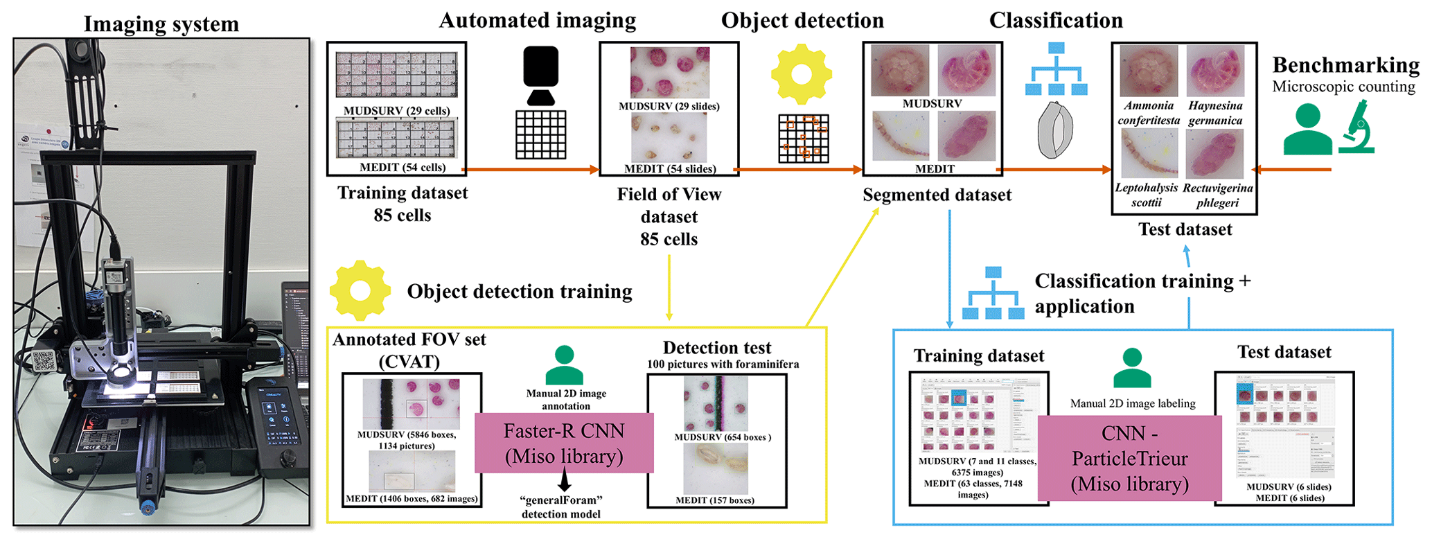
Figure 1 Synthetic workflow (red line) of this study. Automated imaging of micropaleontological slides (with white background) captures multiple foraminifera per field of view (FOV). Bounding boxes for each foraminiferal specimen are detected by a segmentation model (Faster-R CNN, yellow box) trained using the Computer Vision Annotation Tool (CVAT). This step extracts individual foraminifera from FOV images as single-specimen pictures. Specimen labeling (blue box) is performed with the open-source software ParticleTrieur and involves manual verification (green). The final classification models are trained using predefined CNN topologies from the MISO library. The classification models were then applied to independent test samples from each region for comparison.

2.2.2 CNN classification model training

Three classification models were trained, two on the Atlantic MUDSURV low-diversity time series and one on the highly diversified Mediterranean Sea. The MUDSURV intertidal Atlantic samples were used to build the first model, called “MUDSURV species model”, distinguishing the species of foraminifera, regardless of whether the specimens are dead or alive (Rose Bengal-stained). The second model, named “MUDSURV living dead model”, includes two classes for each species, one for living and one for dead specimens, differentiating the staining as well. The third model is the “MEDIT species model”, used for differentiating species from the Mediterranean coast.

Individual images (13 679 images) of foraminifera, obtained from the object detection workflow, were manually labeled using the software ParticleTrieur (version 3.0.5e; GitHub: https://github.com/microfossil/particle-trieur, last access: 18 March 2026) to train a CNN for the automatic recognition of different species (Marchant et al., 2020). Duplicates and images with multiple objects or with blurred, partial, or unrecognizable foraminifera were manually discarded. When possible, manual foraminifera determination based on pictures was performed to species level according to the literature (Barras et al., 2014; Hayward et al., 2020; Jones and Brady, 1994; Jorissen et al., 2023; Milker and Schmiedl, 2012) and reference slides from the Laboratory of Planetology and Geosciences (LPG) at the University of Angers (France). After completion of the dataset's labeling process, the particle/object classification models were trained with the MISO library, containing the scripts to train a CNN and the TensorFlow framework to be able to run machine learning tasks (Marchant et al., 2020; TensorFlow Developers, 2021; GitHub: https://github.com/microfossil/particle-classification, last access: 18 March 2026). ParticleTrieur offers several CNNs to choose from (Marchant et al., 2020) and was run on an HP ENVY x360 Convertible 15 laptop equipped with an AMD Ryzen 7 4700 CPU, 16 GB RAM, and an integrated AMD Radeon Vega 7 GPU. The training of the models was carried out with the foraminifera classes containing more than 10 specimens. A total of 80 % of the dataset was used as “training” to train the model, while the remaining 20 % was grouped into a “validation” dataset and used to evaluate the model performance at each iteration.

Several CNNs proposed by ParticleTrieur were tested, and the best model output for the MUDSURV dataset was obtained using a residual network 50 architecture with transfer learning (ResNet50 TL), while for the MEDIT images, the best results were achieved with a residual network 101 architecture using transfer learning (ResNet101 TL). In both cases, pre-trained weights from the ImageNet database were used, speeding up the training step (He et al., 2015). The ResNet50 TL is a CNN that consists of a total of 50 layers with a special feature that allows it to skip layers if there is a previous strong positive weighting (He et al., 2015). This results in a reduction in gradients, which facilitates classification and makes it possible to form deeper networks with increased accuracy (He et al., 2015). With transfer learning (TL), knowledge already acquired from previous tasks is reused to perform new tasks and facilitate training (Torrey and Shavlik, 2010). Input image sizes are fixed at 224 pixels ($\mathrm{224}\times \mathrm{224}\times \mathrm{3}$) and included color images. Class balancing by weighting was enabled. The epoch (training iterations) size was 10, and the batch size (number of pictures that go through the network in one run) was 32.

Mislabeled images were estimated using a K-NN clustering technique implemented in ParticleTrieur during the first training. Using the estimated mislabeled images, the dataset was revised after a manual check. This process was done once for both MUDSURV and MEDIT, and only labels tagged as misclassified were edited.

2.3 Statistics

Our trained models were used to automatically identify the foraminifera in their respective independent test samples, using a confidence threshold of 0.8. Below this score, individual foraminifera images were labeled as “unsure” and were included in the sample total abundances and taken into account in the faunal parameter calculations (i.e., relative abundances, biotic indices).

To evaluate the potential impact of different classification methods (manual vs. automatic) on ecological interpretations of the Atlantic time series, we compared monthly total foraminiferal abundances, which are indicative of reproduction events.

We calculated the unsure rate for each species, defined as the number of unsure specimens divided by the total specimens of that species, in the Mediterranean test samples. We then compared these rates against the models' training accuracy to assess whether the models' confidence reflects their true performance.

The ecological Tolerant Species Index (TSI-Med; Barras et al., 2014; Parent et al., 2021) was calculated for the Mediterranean samples to assess the ecological quality status (EQS) at the station. Herein, the percentage of tolerant species (%TS_x) is calculated following the list of species by Parent et al. (2021). Using the grain size percentages of the sample, a reference percentage of tolerant species is calculated (%TS_ref; Eq. 1). The TSI-Med is calculated as follows (Eqs. 1 and 2):

$$\begin{array}{}\text{(1)}& {\displaystyle }\mathit{\%}{\mathrm{TS}}_{\mathrm{ref}}=\mathrm{0.1547}\cdot \left(\mathit{\%}\text{grains}<\mathrm{63}\mathrm{\mu }\mathrm{m}\right)-\mathrm{0.3638},\text{(2)}& {\displaystyle }\text{TSI-Med}={\displaystyle \frac{\mathit{\%}{\mathrm{TS}}_x-\mathit{\%}{\text{TS}}_{\mathrm{ref}}}{\mathrm{100}-\mathit{\%}{\mathrm{TS}}_{\mathrm{ref}}}}\cdot \mathrm{100}.\end{array}$$

3 Results

3.1 Object detection

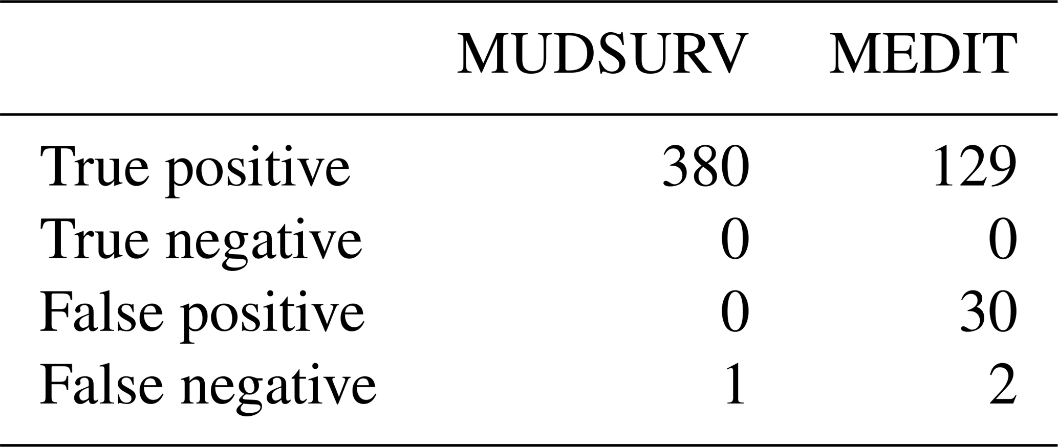
A total of 100 pictures from micropaleontological slides, per studied region, were viewed after completing the inference of the “generalForam” segmentation model. However, additional non-foraminifera particles, glue residues, and boundary lines within the slides were also considered particles by the model and therefore segmented and counted. Out of 381 foraminifera specimens across 100 images from the MUDSURV micropaleontological slides, only 1 specimen was not recognized as a foraminifera (Table 1), yielding an accuracy and recall of 99.74 %, precision of 100 %, and an F₁ score of 0.99. In the MEDIT micropaleontological slides, out of the 131 foraminifera specimens on 100 images, 129 were correctly identified as such, and 2 were missed (Table 1). The model identified 30 false positives, yielding a precision of 81.11 % and an accuracy of 80.12 %. The recall is the highest (98.47 %), with only two foraminifera missed by the model. Overall, the F₁ score is 0.89.

Table 1 Validation of the object detection: 100 pictures from both regions including foraminifera were observed to assess detection performance using the Computer Vision Annotation Tool (CVAT).

3.2 MUDSURV classification models

3.2.1 MUDSURV classification model training

After the segmentation, the resulting dataset consisted of 6388 images of individual (living and dead) foraminifera showing four dominant calcareous species with similar spiral shell shapes (trochospiral for Ammonia confertitesta and planispiral for Elphidium oceanense, Elphidium selseyense, and Haynesina germanica) and two additional less abundant species: one agglutinated with an initial planispiral turn followed by a uniserial shell (Ammobaculites balkwilli) and one monothalamid species (Psammophaga sp.) (Appendix A). Finally, four very rare species, represented only by a few images (< 10), were not included in the training set: Ammotium salsum (n=5), Lagena sp. (n=3), Leptohalysis scottii (n=1), and Quinqueloculina sp. (n=4), yielding a final dataset of 6375 foraminifera images (Appendices A and C).

This image dataset was used for both models (species with or without a living/dead distinction); only the labels differed according to the purpose of the model: (i) the first model (MUDSURV species model) distinguished the different species (Fig. 2), and (ii) the second model (MUDSURV living dead model) distinguished the different species and included an indication of whether they were living or dead specimens according to the staining.

The MUDSURV species model, intended to distinguish the six different species (i.e., six classes), shows an accuracy of 96.0 %, a precision of 96.1 %, a recall of 95.5 %, and an F₁ score of 95.8 % (Fig. 2; Appendices C and D). Five of the six species are recognized with an accuracy of over 96 %, while Ammobaculites balkwilli and Psammophaga reach 100 %. Three of the dominant species reach an accuracy around 96 %–98 %, namely Ammonia confertitesta, Elphidium oceanense, and Haynesina germanica. Elphidium selseyense (104 specimens) has the lowest accuracy (83 %), showing the highest misidentifications with the species Ammonia confertitesta (9 %) and Elphidium oceanense (7 %) (Fig. 2). For the MUDSURV species model, 61 foraminifera were mislabeled (0.96 %).

The MUDSURV living dead model, designed to distinguish the different species and their vital status defined by the RB stain, achieves an accuracy of 94.2 % for 10 different classes (see Fig. 2; Appendices C and E). This results in a precision of 91.5 %, a recall of 93.7 %, and an F₁ score of 92.2 (Fig. 2). Herein, 8 of the 10 classes are recognized with an accuracy of over 90 %. The Ammonia confertistesta dead specimen (101 specimens) class shows an accuracy of 80 %, followed by the Elphidium dead specimen class with an accuracy of 86 % (66 specimens), the only two classes being under 90 %. All Psammophaga sp. specimens (n=2) were misclassified as dead. Of the dead Ammonia confertitesta, 14 % were classified as alive with the CNN, and, in contrast, 6 % of living Elphidium were classified as dead. Between the Elphidium species, 7 % of Elphidium selseyense were wrongly classified as Elphidium oceanense and vice versa for an extra 3 %. For the MUDSURV living dead model, 138 foraminifera were mislabeled (2.16 %). The MUDSURV species model was trained in 540 s and the MUDSURV living dead model in 600 s.

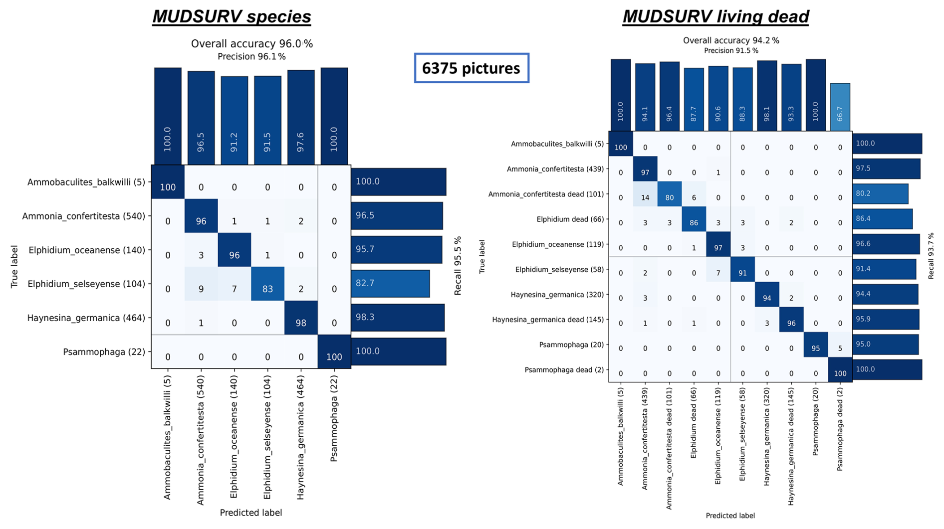
Figure 2 Confusion matrices of the two classification CNN models trained on the MUDSURV Atlantic dataset (6375 pictures of 6 species). Each row represents the actual class with percentages, and the diagonal values (top left to bottom right) show the proportion of correctly classified specimens. Off-diagonal values indicate misclassifications. Left panel: MUDSURV species model at the species level (accuracy: 96.0 %, precision: 96.1 %, recall: 95.5 %). Right panel: MUDSURV living dead model combining the species level and the vital status (Rose Bengal staining) (accuracy: 94.2 %, precision: 91.5 %, recall: 93.7 %).

3.2.2 MUDSURV model testing

To verify the applicability of the MUDSURV species model, six independent test samples from MUDSURV (monthly monitoring, October 2020 to April 2021, except February 2021) with a minimum of 145 (B-01/21) and a maximum of 1650 (B-10/20) specimens were used (Appendix A). The number of foraminifera per species counted manually was compared with the number automatically counted using the CNN model for each station (Fig. 3). Overall, the CNN correctly identifies 91.48 % of the specimens on average. This value ranges from 85.11 % for the January 2021 sample to 93.34 % for the October 2020 sample. The absolute densities of the four major species exhibit similar temporal trends between monthly samples for human and CNN analyses (Fig. 3). For Ammonia confertitesta and Haynesina germanica, the absolute densities are similar between both approaches, whereas they are slightly different for the Elphidium species, especially for E. selseyense, which also exhibited lower accuracy according to the model performance (Figs. 2, 3). When a difference is noticed, this is mostly the CNN that underestimates the absolute density of the species. This is mainly due to the classification of specimens in the “unsure” class when the threshold of 0.8 is not reached.

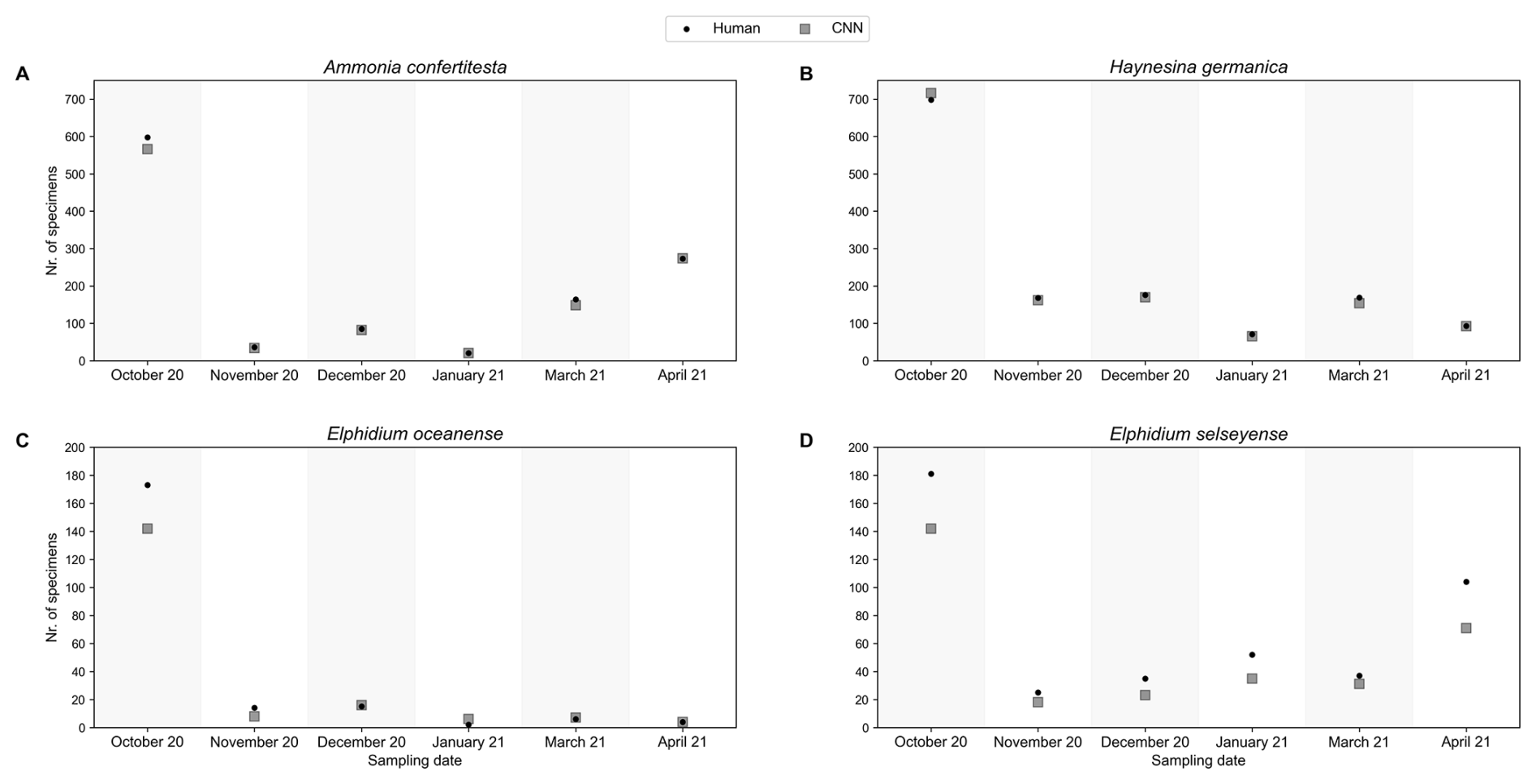
Figure 3 Comparison of the human-based (point) vs. automatic (CNN MUDSURV species model, threshold 0.8, square) counts of the four main species from the low-diversity MUDSURV environment (Station B, October 2020 to April 2021, except February 2021). (a) Ammonia confertitesta, (b) Haynesina germanica, (c) Elphidium oceanense, and (d) Elphidium selseyense.

3.3 MEDIT

3.3.1 MEDIT model

The dataset for the Mediterranean region comprises a total of 7291 images of individual foraminifera out of which 7148 were used for the CNN training (species with fewer than 10 pictures were discarded) of 63 species of foraminifera, which correspond to the 63 classes defined in the model (Appendices A, C, and F). The training of the MEDIT species model took 873 s.

The MEDIT species model reaches an accuracy of 82.2 % in species recognition. It achieves a precision of 77.3 %, a recall of 70.5 %, and an F₁ score of 72.3 (Fig. 4). More than half of the species (40 classes) reach an accuracy of over 70 %. For 10 of them, the accuracy lies between 70 %–80 % and for an extra 15 species between 81 %–90 %, while 16 species are recognized with an accuracy > 90 %. Finally, a total of seven species are recognized with 100 % accuracy. Identification rates of 100 % were achieved for Ammodiscus planus, Cornuspira foliacea, Nonion scaphum, Nonionella turgida, Spiroloculina grateloupi, Trochamminula, and Valvulineria bradyana. In contrast, a total of 12 species present an accuracy below 50 %, with Biloculinella irregularis, Miliolinella subrotunda, and Quinqueloculina spp. completely unpredicted by the model (accuracy = 0 %). For the MEDIT species model, 918 foraminifera were mislabeled (12.84 %).

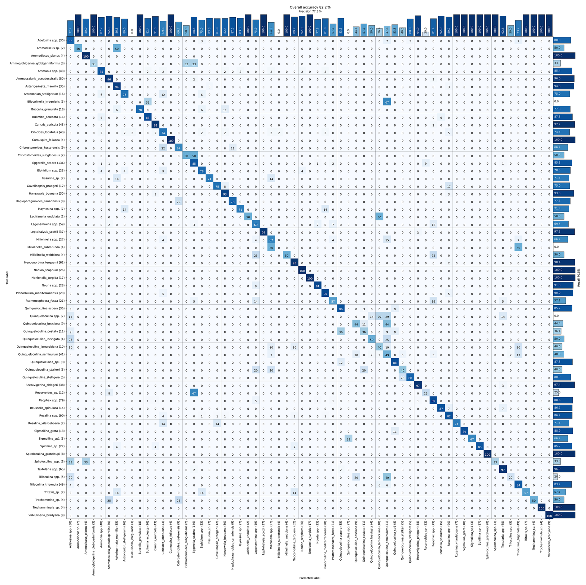
Figure 4 Confusion matrix of the MEDIT species model. Each row represents the actual class with percentages, and the diagonal values (top left to bottom right) show the proportion of correctly classified specimens. Off-diagonal values indicate misclassifications; 7148 pictures of 63 classes were used for the training. Overall accuracy: 82.2 %, precision: 77.3 %, recall: 70.5 %, F₁ score: 72.3.

3.3.2 MEDIT model testing

The MEDIT model above was applied to the six “independent test samples” (Appendices A and G) to compare its identification with an expert ground truth. The foraminiferal abundance in samples ranges from 36 to 327 specimens. The accuracy of correct predictions of the model spans 63.75 % (mid, September 2014) to 79.26 % (proximal, May 2014), with an average value of 69.69 %. Two species were present in the test samples but were not identified as a class in the model since they were absent from the training set (Fursenkoina acuta and Cassidulina oblonga). Figure 5 shows the comparison between human counts and CNN predictions for the four most common taxa in the test samples (Eggerella scabra, Reophax sp., Rosalina sp., and Textularia sp.). Overall, the CNN prediction follows similar trends to human counts across all samples, although discrepancies in magnitude occur.

Out of a total of 28 species declared as tolerant in Parent et al. (2021), 8 were present in the test samples. Of the six samples analyzed by the CNN, only one resulted in an EQS different from the expert assessment (Fig. 6). In sample ref. 05/14, the EQS changes from “very good” to “good” after the CNN classification (Fig. 6).

A general trend where higher training accuracy is associated with lower uncertainty (number of unsure specimens of a species divided by total specimens of this species) is observed in Fig. 7, although this relationship is not strictly linear. Several species with high accuracy (above ∼ 85 %) exhibit low unsure rates, indicating confident model predictions when sufficient training performance is achieved. Larger bubble sizes (representing more images) are mostly concentrated in this high-accuracy, low-uncertainty region, suggesting that greater data availability improves both accuracy and confidence. Seven species have unsure rates of 100 %. Two of them were not present in our dataset (Fursenkoina acuta (11) and Cassidulina oblonga (15)), having an unsure rate of 100 % and accuracy of 0 %. Cassidulina oblonga, being notably a tolerant species, was used to calculate for the TSI-Med. On the other hand, two species reach unsure rates of 100 % but have accuracies of over 80 % (Reussella spinulosa (18) and Asterigerinata mamilla (22)). Additionally, several species with moderate accuracies (40 %–70 %) display relatively high unsure rates (40 %–60 %), suggesting transitional performance.

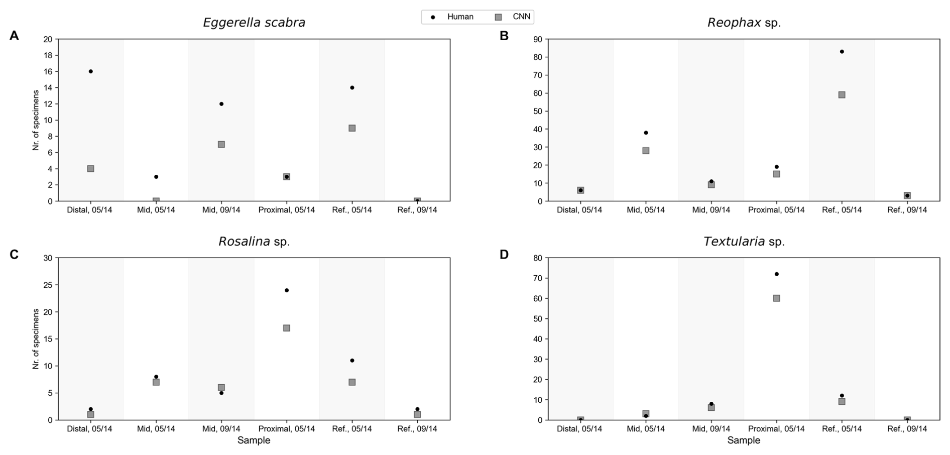
Figure 5 Comparison of the human-based (point) vs. automatic (CNN MEDIT species model, threshold 0.8, square) counts of the four main species from the high-diversity environment MEDIT along a sewage outlet from distal to proximal. (a) Eggerella scabra, (b) Reophax sp., (c) Rosalina sp., and (d) Textularia sp.

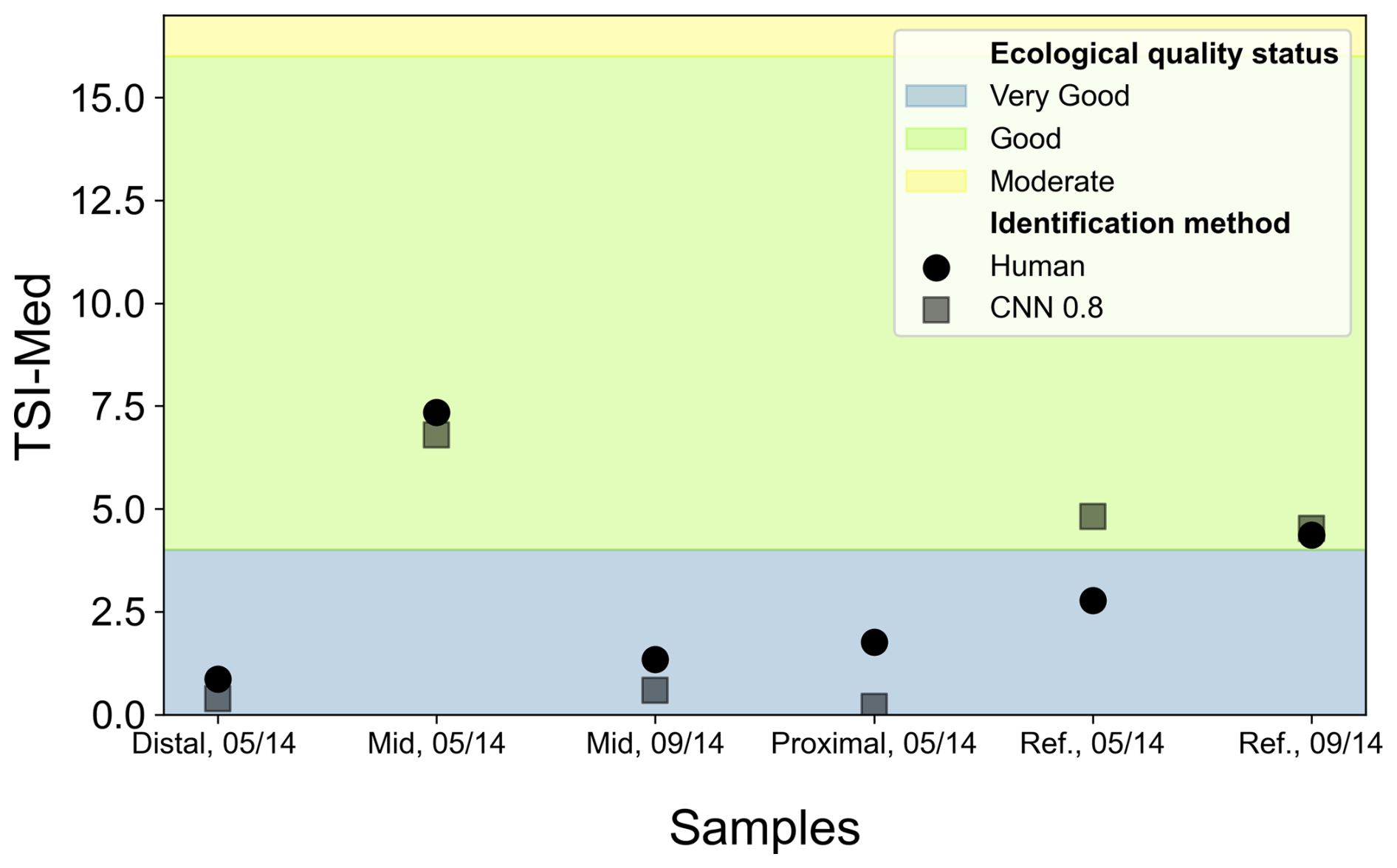
Figure 6 Comparison of the TSI-Med results derived from the human (points) and automatic (CNN MEDIT species model, threshold 0.8, square) counting along a sewage outlet from distal to proximal. Ecological quality status is displayed by the color code: blue, green, and yellow for “very good”, “good”, and “moderate” status, respectively (Parent et al., 2021).

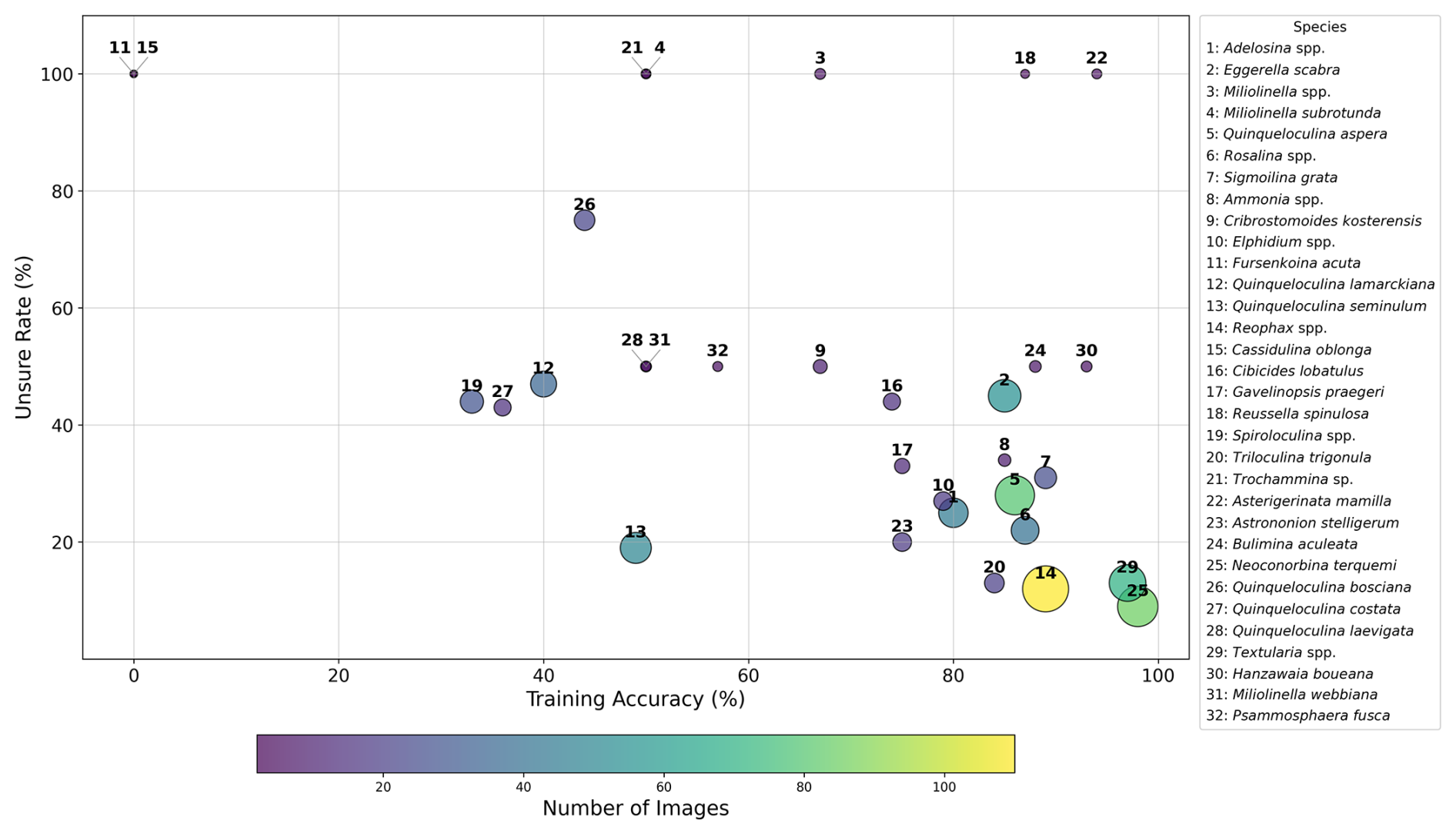
Figure 7 Relationship between training accuracy and unsure rate (unsure specimens divided by the total specimens of that species) across species present in Mediterranean test samples. Each point represents a species (numbered 1–32; see legend), with the bubble size and color-coding proportional to the number of test images available for that species.

4 Discussion

Overall, CNN-based solutions for the identification of foraminifera (species, Rose Bengal-stained) show promising results in the two locations studied, although higher accuracies are achieved in environments with lower diversity. This is the first time that a model on benthic foraminifera has been trained to identify living foraminifera and a large quantity of species.

Generally speaking, using the Sashimi approach is faster than manually identifying living foraminifera under a microscope. Scanning a single micropaleontological slide is done in about 1.5 h, and applying the already-developed models with ParticleTrieur to obtain the final identification of a foraminiferal dataset takes less than a minute (depending on the size of the dataset). Right now, our approach is limited to micropaleontological cells, where the foraminifera have previously been picked and glued. As a next step, focusing on scanning sieved raw samples would make hand picking foraminifera unnecessary while leading to faster identification, yet it would imply a recognition of all the objects in the sediments. This would involve either pre-sorting foraminifera from particles using an additional model or increasing the number of classes during the training part in ParticleTrieur.

4.1 Object detection

For the object detection, recall (i.e., the number of false negatives) is the most important metric because the primary objective is to ensure that all foraminifera are detected. Missing true specimens results in information loss, which is particularly needed when analyzing living faunas. While the model produced false positives from glue residues, grid lines, and other non-foraminiferal particles, these will be corrected in the classification step process. The high recall values demonstrate that the approach minimizes missed specimens and maximizes the reliability of the dataset.

4.2 Composition of the training dataset of the identification models

Our results show that a small number (∼ 50) of species-specific pictures is sufficient for the MUDSURV models to reach high accuracies if the considered species present significant morphological differences compared to other species considered. For example, 24 and 112 pictures of Ammobaculites balkwilli and Psammophaga, respectively, were enough to train the MUDSURV species model. Previous studies dealing with automatic identification of foraminifera have found lower model accuracies with a higher total number of images and images per species (Adebayo et al., 2023; Hsiang et al., 2019; Marchant et al., 2020), showing that distinct morphologies throughout the dataset allows the use of a minimal training set (e.g., Ammobaculites balkwilli in MUDSURV, Valvulineria bradyana in MEDIT). Species that have a unique morphology achieve significantly better accuracies (Marchant et al., 2020).

The average accuracy for the test samples from the Mediterranean is ∼ 69.7 %. CNN-based results were compared to the numbers of manually identified and counted samples under a stereomicroscope. The presence of taxa in the picked samples for which the model was not trained (e.g., Brizalina difformis, Laevidentalina haueria, Pyrulina fusiformis) leads to a significantly lower accuracy. The CNN was thus not designed to identify these foraminifera. For instance, Brizalina difformis was predicted as Textularia spp. due to similar general morphology.

Additional images per species should nevertheless be scanned to optimize the model for species that share close morphological patterns, as well as for species scarcely represented in the dataset, which were discarded due to an insufficient number of pictures necessary for training (< 10). The results of both models show that the number of training specimens is important for the identification. A higher number of training pictures yields higher possibilities for accurate identifications. The creation of a general model, location independent, would be ideal; however, it may be difficult to implement due to different working standards in different institutes and taxonomic expertise. Classes that perform well during model validation also tend to achieve high accuracy when applied to independent test samples, confirming the models' reliability (Marchant et al., 2020).

The observed relationship between accuracy of a species and unsure rate (Fig. 7) indicates that, although improved classification performance is often associated with increased model confidence, these two metrics are not strictly coupled. Species represented by fewer test images may show greater variability, including higher proportions classified as unsure or lower accuracies. The presence of species with high accuracy but maximal unsure rates points to inconsistent model confidence, potentially due to intra-class variability or similarity with other taxa. Conversely, species with low accuracy and elevated unsure rates likely reflect ambiguous morphological features (e.g., porcelaneous foraminifera). Overall, these results highlight that unsure rates provide complementary information to accuracy, revealing ambiguities in model predictions not captured by accuracy alone.

4.3 Identification based on morphology

Although the benthic foraminifera in the MUDSURV dataset share the same outline morphology (Hayward et al., 2020), the identification is successful, with minor misclassifications (e.g., Ammonia confertitesta and Elphidium selseyense). Misinterpretations are made due to low-quality pictures, highlighting the limitation of the imaging setup, including the 5-megapixel camera used. Switching to a camera and associated optics with a better resolution will probably improve the results but will come with a computing trade-off, requiring more time to be processed (uploading and downloading data for object detection etc.).

When looking at the misclassified images of the CNN, it is noticeable that some foraminifera are oriented with specific diagnostic features such as coiling and aperture being poorly visible, leading to incorrect predictions (Marchant et al., 2020). This is especially true for the Elphidium species specimens. In some images, foraminifera are discolored, rendering it difficult to recognize their features. Nevertheless, these images also include specimens that were mislabeled in retrospect, and an expert bias cannot be denied, as it is a matter of supervised learning, based on the personal level of knowledge and experience of the user (Al-Sabouni et al., 2018; Fenton et al., 2018). Al-Sabouni et al. (2018) and Fenton et al. (2018) concluded that benthic foraminifera exhibit morphological differences when observed from the spiral versus the umbilical side, making it necessary to have enough pictures of both views of the same species (Fig. 8a–b). Another possibility would be to create distinct classes for both the umbilical and the spiral sides of benthic foraminifera. While feasible, this approach could result in a combinatorially high number of classes, making the classification scheme more complex and harder to manage. Labeling 2D images can introduce errors due to experts not having access to both views of all parts of the shell (in contrast to manually manipulating specimens under a microscope) but appears to be able to capture broad trends in the data (Austen et al., 2018).

Accuracy of species identification generally increases with the number of training images, particularly for species that are morphologically distinct from others. Conversely, identification accuracy tends to decrease when multiple species from the same genus (e.g., several porcelaneous species) are included, likely due to their morphological similarity (Marchant et al., 2020). Distinct characteristics of a species reduces the number of pictures that are needed to train the model. It is particularly noticeable that the CNN has difficulties in distinguishing the different miliolid (porcelaneous test) foraminifera (Fig. 8e–h). The common practice of using micropaleontological slides with a white background, which aids in color differentiation when working with Rose Bengal-stained specimens under a binocular microscope, appears to be suboptimal in our imaging workflow. Species of the genera Quinqueloculina, Spiroloculina, and Triloculina are therefore confused with other porcelaneous species like Adelosina spp. in the MEDIT database. The morphological features necessary for their determination at the species level are often hardly visible on the images (Fig. 7e–h). For several species of the genus Quinqueloculina, the accuracy of correctly identified foraminifera is usually less than 50 %. Only Quinqueloculina aspera stands out with 74 % accuracy, most probably due to the agglutinated texture of its miliolid shape shell. Yet, Fenton et al. (2018) showed that between experienced identifiers, the median accuracy is around 79 % for the cross-recognition of planktonic foraminifera, an accuracy not that far from the worst species identified by our CNN. In summary, to overcome the problems of miliolid identification and distinguishing living from dead foraminifera, micropaleontological slides with a different background color should be tested in the future. Previous studies have used micropaleontological slides, cups, or trays, with a black background (Hayat et al., 2026; Hsiang et al., 2019; Marchant et al., 2020; Mitra et al., 2019), but these studies focused on fossil faunas and therefore did not aim to distinguish between living and dead foraminifera.

The MEDIT species model exhibits limitations in resolving taxonomic distinctions among various agglutinated foraminifera. They are often misidentified due to their morphology and color. For example, there is a risk of confusion between Cribrostomoides kosterensis and Haplophragmoides canariensis and between Lagenammina sp. and Reophax sp. (Fig. 8i–l). For the first example, the differentiation between these agglutinated species is difficult; indeed, Cribrostomoides is planispiral, and Haplophragmoides is trochospiral, and these features often require direct manipulation under the stereomicroscope for accurate identification. Lagenammina sp. and Reophax spp. are also often misidentified, with Lagenammina sp. often classified as single chambers of Reophax scorpiurus.

The model's predictions become more uncertain as the number of classes that are morphologically similar increases, especially when foraminiferal features are not recognizable on the image. For trochospiral individuals, images of both the spiral and the umbilical sides must be used in the dataset to train the model (Marchant et al., 2020). This in turn ensures that the label extracts several features of a class, which can potentially lead to complications. One possible solution would be to create several classes that each represent the umbilical or spiral side. However, an increased number of classes and variables makes identification more complex and difficult (He et al., 2015; Marchant et al., 2020). While this study suggests that the use of CNN-based models can be used to identify living benthic foraminifera, they still require complementary expert taxonomic knowledge for accurate image classification, particularly when processing 2D digital images (Al-Sabouni et al., 2018; Zhong et al., 2017).

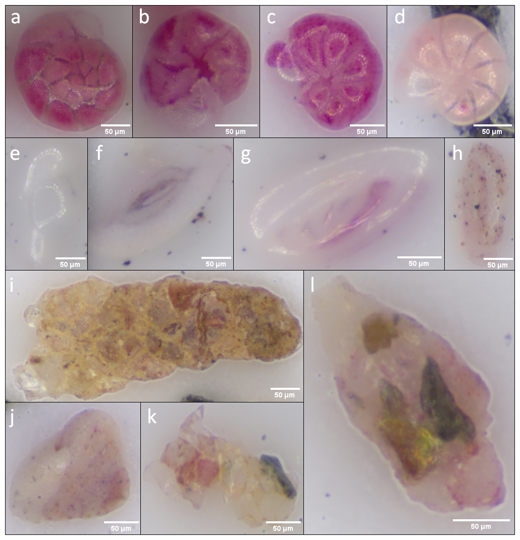
Figure 8 (a–b) Spiral (a) and umbilical (b) view of Ammonia confertitesta. The CNN has to recognize both of the sides as the same species and also from every angle. (c–d) Degradation of Rose Bengal staining in Haynesina germanica from the Atlantic time series (MUDSURV), complicating the CNN recognition of living specimens. Panel (c) shows a specimen with a bright pink color, indicating that it was alive at the sampling time (preserved until scanning in ethanol), while (d) RB staining is faded even though it was considered alive at picking time (sampling in 2016 preserved in ethanol, dried in 2017). (e–h) Porcelaneous foraminifera showing the limited visibility of whitish shells on white background. (e–f) Adelosina spp., (g) Quinqueloculina aspera, and (h) Quinqueloculina bosciana. (i–l) Agglutinated foraminifera: (i) Ammosclaria pseudospiralis, (j) Textularia spp., (k) Reophax spp., and (l) Lagenammina spp., showing that an assumption on the vital status is not trivial, though for the left specimen, RB staining is visible, but determining if it is inside/outside is difficult. (k–l) Misclassifications can also occur throughout agglutinated species because of their similar appearance through their composite material.

4.4 Recognition of living and dead tests of the same species

Of particular importance in assessing the ecological status of marine sedimentary environments is the determination of the vital status of foraminifera through the RB staining used in marine biomonitoring studies (Schönfeld et al., 2012). Pronounced visible RB staining is easier to handle for the CNN and will provide better results in the automatic identification of the stained foraminifera. Because the staining will fade with time once the specimen is stored and dried in the micropaleontological slides, scanning of foraminifera should be processed as fast as possible after picking to obtain good pictures (Fig. 8). The staining from samples of intertidal Atlantic time series is often very good in comparison to our Mediterranean samples. In the Mediterranean samples, the overall staining is not very pronounced, preventing us from identifying living specimens.

Individuals of Ammonia confertitesta from the mudflat samples (MUDSURV) were considered alive by the human expert when cytoplasm was visible through all but the last one to four chambers. These individuals did not necessarily show strong coloration (Bernhard, 2000), which led to misidentification of living and dead specimens by the CNN. In general, species recognition remained easier than the vital state determination (dead or alive) of the specimen. This seems to be, at least partly, a result of human bias through inconsistent labeling of the training set based on stained foraminifera and shows the importance of freshly sieved samples with well-preserved foraminiferal tests (Bernhard, 2000).

RB-stained foraminifera (containing species with various shell textures) from the Mediterranean samples are less easy to identify in comparison to the ones from MUDSURV (containing mainly hyaline tests), which is also why for the Mediterranean samples only a species model was developed. This is a typical problem for miliolid foraminifera where the coloration is often easily visible through the shell when the individual is in a solution, but the staining becomes less detectable when the specimen is dry (Parent et al., 2021). If foraminifera are maintained under wet conditions, the distinction between living and dead specimens is achieved more easily. For that reason, miliolid foraminifera are often wet or broken when hand-picked by humans (Fig. 8; Parent et al., 2021). This cannot be applied to automatically photographed individuals and consequently to the determination made by the model.

4.5 Implications for ecological interpretations

4.5.1 Low-diversity intertidal study area

To evaluate the potential of automated foraminiferal identification in ecological studies, we first focus on low-diversity intertidal environments, where species dynamics are well-documented and can be linked to environmental variability. In the case of the Bourgneuf intertidal mudflat assemblages, Choquel et al. (2026) used species absolute abundances in order to study foraminiferal dynamics through time according to environmental parameters. In particular, reproduction events (high-density events) were counted every time a species' abundance exceeded a certain limit. Benthic foraminifera reproduction follows a change of generation every few months in sexual and asexual phases (Murray, 2006). These reproduction events can be influenced by environmental factors, and because only the > 150 µm fraction is analyzed, a time lag occurs between the actual reproduction and observation in samples (Schönfeld et al., 2012).

The threshold value for a reproduction event was determined to be above 600 living foraminifera per 50 cm³ for Ammonia confertitesta, Elphidium oceanense, and Haynesina germanica and above 100 foraminifera per 50 cm³ for Elphidium selseyense (Choquel, 2026). In the period from October 2020 to April 2021, three high-density events could be observed (Fig. 3). Elphidium selseyense high-density events occurred in October 2020 and April 2021 (Fig. 3). In October 2020, a high-density event took place for Haynesina germanica (Fig. 3). Both of the high-density events which occurred in October 2020 could be identified using the CNN model with an accuracy of 67 % (Fig. 3).

In this case study based on low-diversity assemblages, we can therefore attest that the CNN model is able to reach sufficiently good results to study the seasonal dynamics of the different foraminiferal species. Fully automating the analysis of monitoring studies would enable increasing the sampling frequency to monthly or bi-monthly intervals, allowing a better understanding of foraminiferal responses to environmental changes in this kind of highly dynamic environment. The FOBIMO-group (Schönfeld et al., 2012) developed an international protocol for biomonitoring studies, recommending that sampling should be done once a year, preferably in autumn. To capture the variability of the environment, three replicates are necessary, yielding three samples for one station (Schönfeld et al., 2012). Most biomonitoring studies comprise several stations that are sampled seasonally or monthly, leading to an overwhelming number of samples (Alve et al., 2016; Bouchet et al., 2007; Burone et al., 2007; Dubois et al., 2021; Kenigsberg et al., 2020; Morvan et al., 2004). An automated approach saves time, enables the processing of larger sample sets, and increases the amount of data available on environmental dynamics while also improving taxonomic consistency by reducing operator-dependent bias.

4.5.2 High-diversity coastal study areas

We then assess the applicability of the automated identification model in more complex, high-diversity coastal environments, where ecological indices such as TSI-Med are used to evaluate ecosystem quality (Barras et al., 2014; Cavaliere et al., 2021; Dubois et al., 2021; Parent et al., 2021). Despite an average accuracy of ∼ 60 % for the correct identification of the Mediterranean test foraminifera, the TSI-Med index, on the test dataset, shows almost no differences in the evaluation of ecosystem quality between the manual and automatic methods (Fig. 6). Unlike other indices, such as diversity indices (Bouchet et al., 2012) or Foram-AMBI (Jorissen et al., 2018), the TSI-Med requires only the identification of a limited number of species listed as tolerant to environmental stress and the accounting of the total number of living foraminifera. Our findings indicate that taxa assigned as tolerant according to Parent et al. (2021) are among those yielding good accuracies as enough training pictures were available. Examples include Cancris auricula and Leptohalysis scottii. The human–machine comparison of the TSI-Med values shows reliable automated results, indicating that the combination of automated identification and TSI-Med calculation could be applied in studies of the ecosystem quality. To confirm this result, it would be interesting to test the model on samples including more species listed as tolerant since only 8 out of 28 were present in our samples. For Foram-AMBI (Alve et al., 2016; Bouchet et al., 2021; Jorissen et al., 2018), all species would need to be correctly identified with the CNN to obtain a correct value since all species are classified into five different ecological groups from sensitive to opportunist. Rare species would also need to be identified, which would be more difficult due to the limited number of images available to properly train the CNN.

4.5.3 Scientific and practical implications

The use of machine learning for the automated identification of benthic foraminifera has the potential to substantially transform current analytical workflows. Taxonomic identification remains one of the main issues in foraminiferal studies, as it requires time and specialized expertise. It is important to note that the reliability of CNN models is built upon hundreds to thousands of expertly labeled images, underscoring that such approaches depend on the essential role of taxonomists.

By enabling rapid and consistent species-level classification from large image datasets, the approach presented here could significantly reduce the processing time and facilitate the analysis of larger sample sets and higher-temporal-resolution datasets. When combined with automated imaging, such as the modified 3D printer setup used in this study, CNN models could contribute to the development of integrated, high-throughput systems for the analysis of benthic foraminiferal assemblages. Such systems would enhance the practicality of using foraminifera as bioindicators in environmental monitoring programs, where rapid and standardized assessments are increasingly needed.

5 Conclusions

Our method, based on automatic image acquisition and AI, shows the potential and significant benefit of using convolutional neural networks (CNNs) to streamline the identification of living benthic foraminiferal species in biomonitoring studies. This approach appears to be more efficient in low-diversity ecosystems than in high-diversity ecosystems, where the morphological space is often more complex.

This development tackles the need for long-term and high-temporal- and high-spatial-resolution studies that are time-consuming in terms of technical work but also face the problem of operator taxonomic bias. This would finally help to promote the use of foraminifera as bioindicators in regulations, allowing us to obtain faster and more reliable information about the health and ecological status of our oceans and coastal environments.

Appendix A

Table A1 Sample overview. All samples shown in regular font were used for the training of the models. Samples shown in bold were used for the segmentation training with CVAT, while the independent test samples are shown in italic. ^* indicates raw samples scanned. MEDIT: SCM Emi P, SCM Emi M, and SCM Emi L correspond to proximal, mid-site, and distal locations, respectively, relative to the sewage outlet.

Appendix B

Figure B1 Example of image fusing.

Appendix C

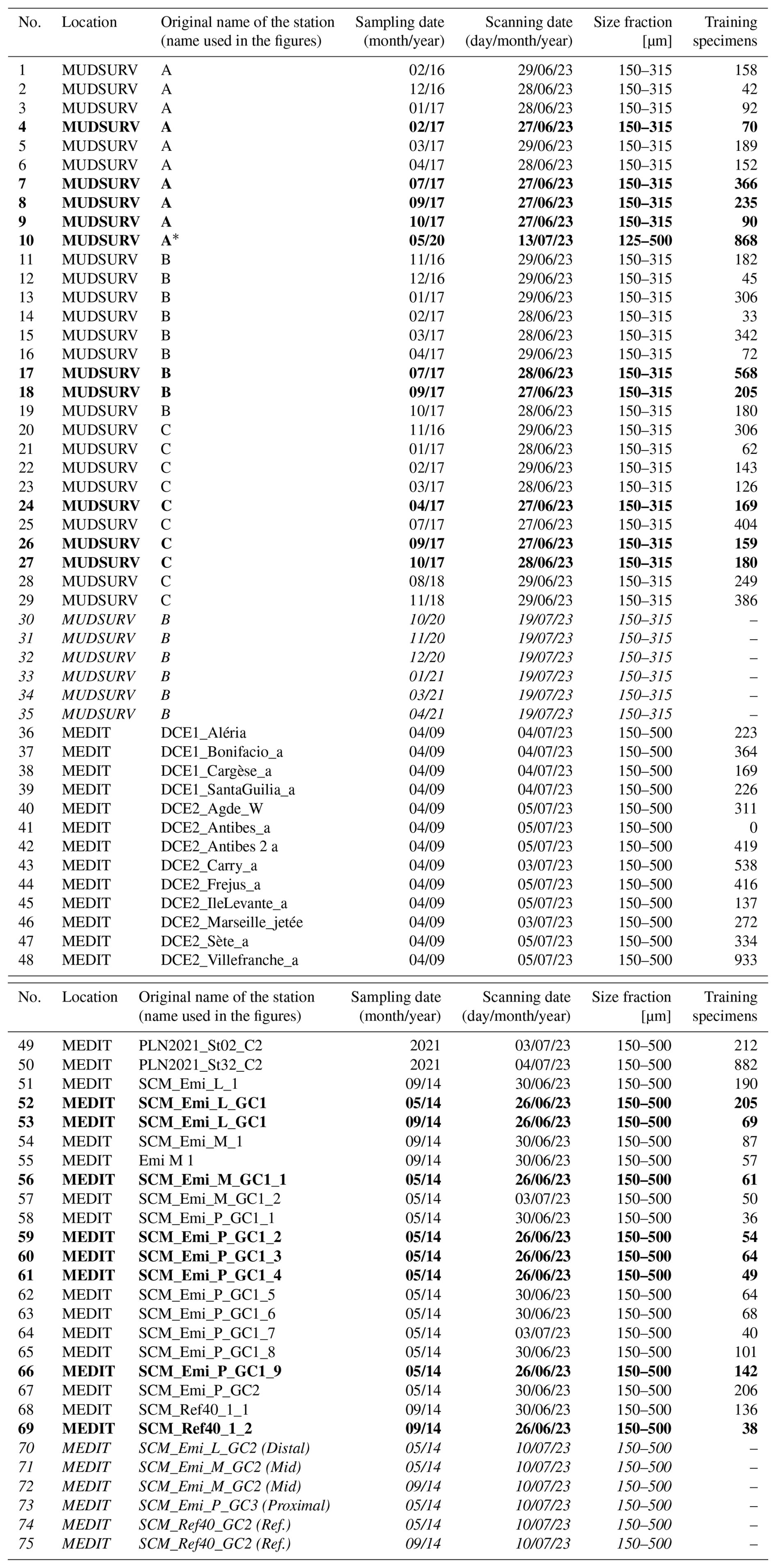
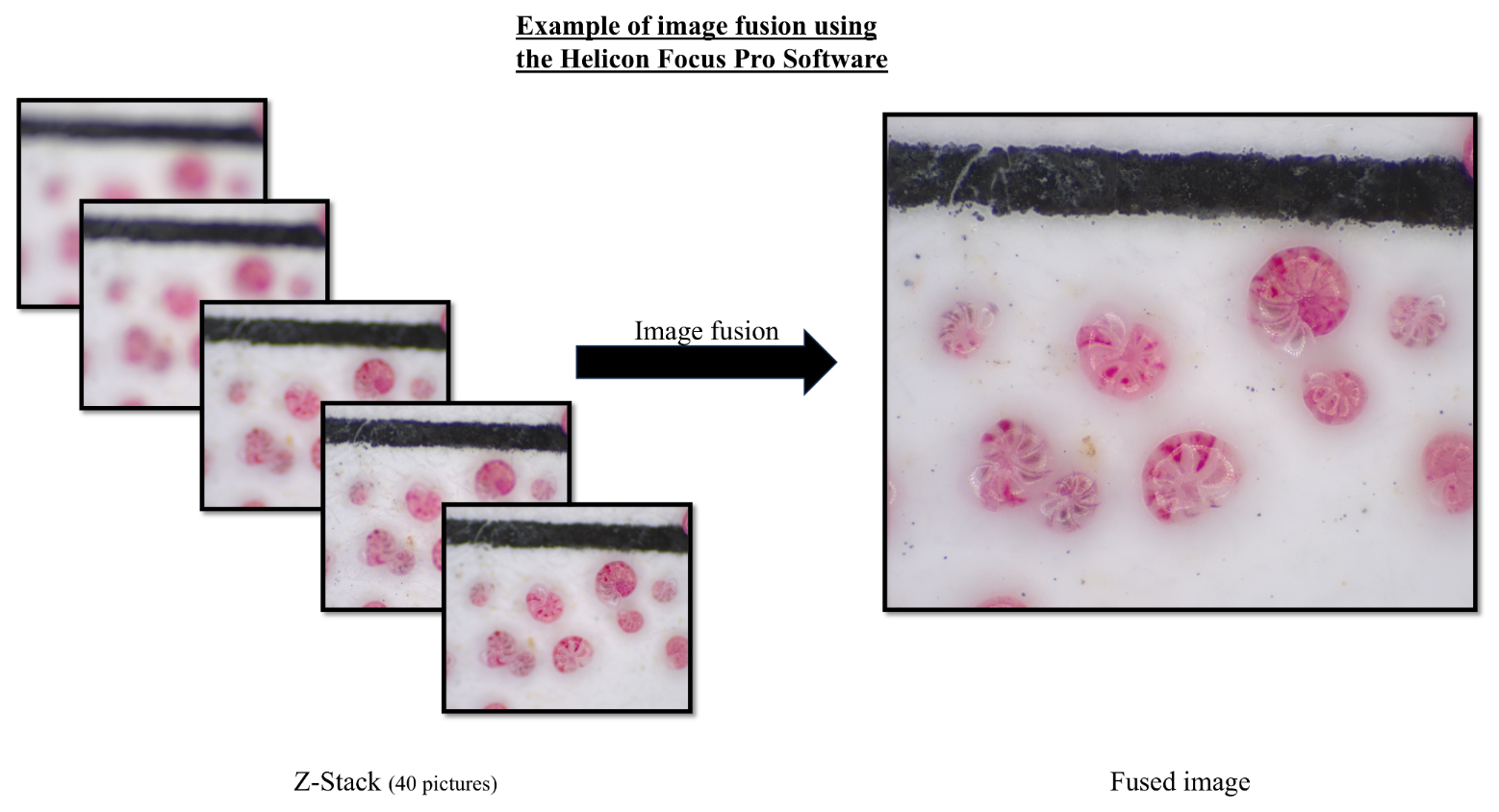
Table C1 Classes and number of pictures for each species in the training dataset of the MUDSURV species/living dead models and the MEDIT species model; ^* indicates that this species was not used for training because fewer than 10 pictures were available.

Appendix D

Table D1 Metrics of the MUDSURV species model after training.

Appendix E

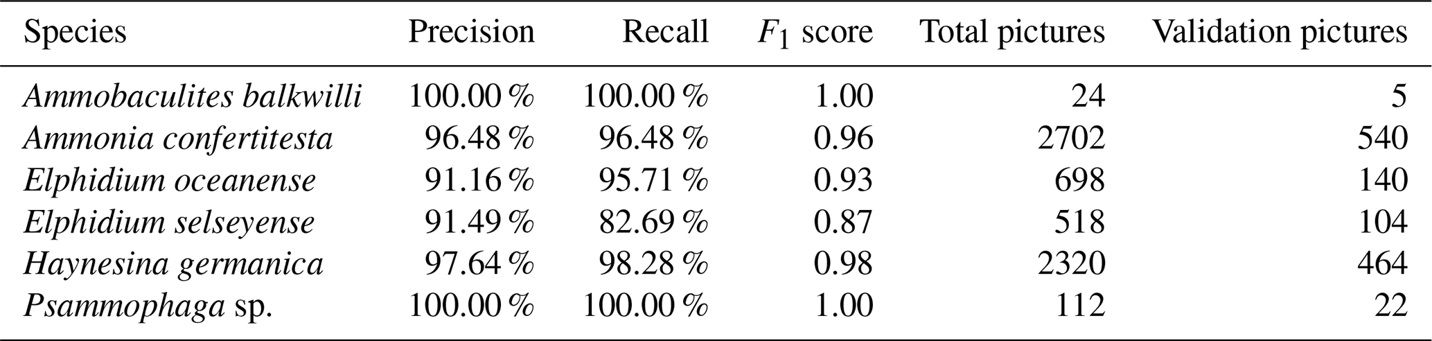
Table E1 Metrics of the MUDSURV living dead model after training.

Appendix F

Table F1 Metrics of the MEDIT species model after training.

Appendix G

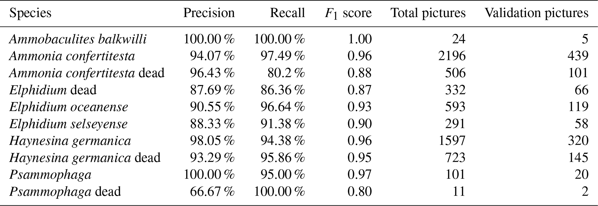
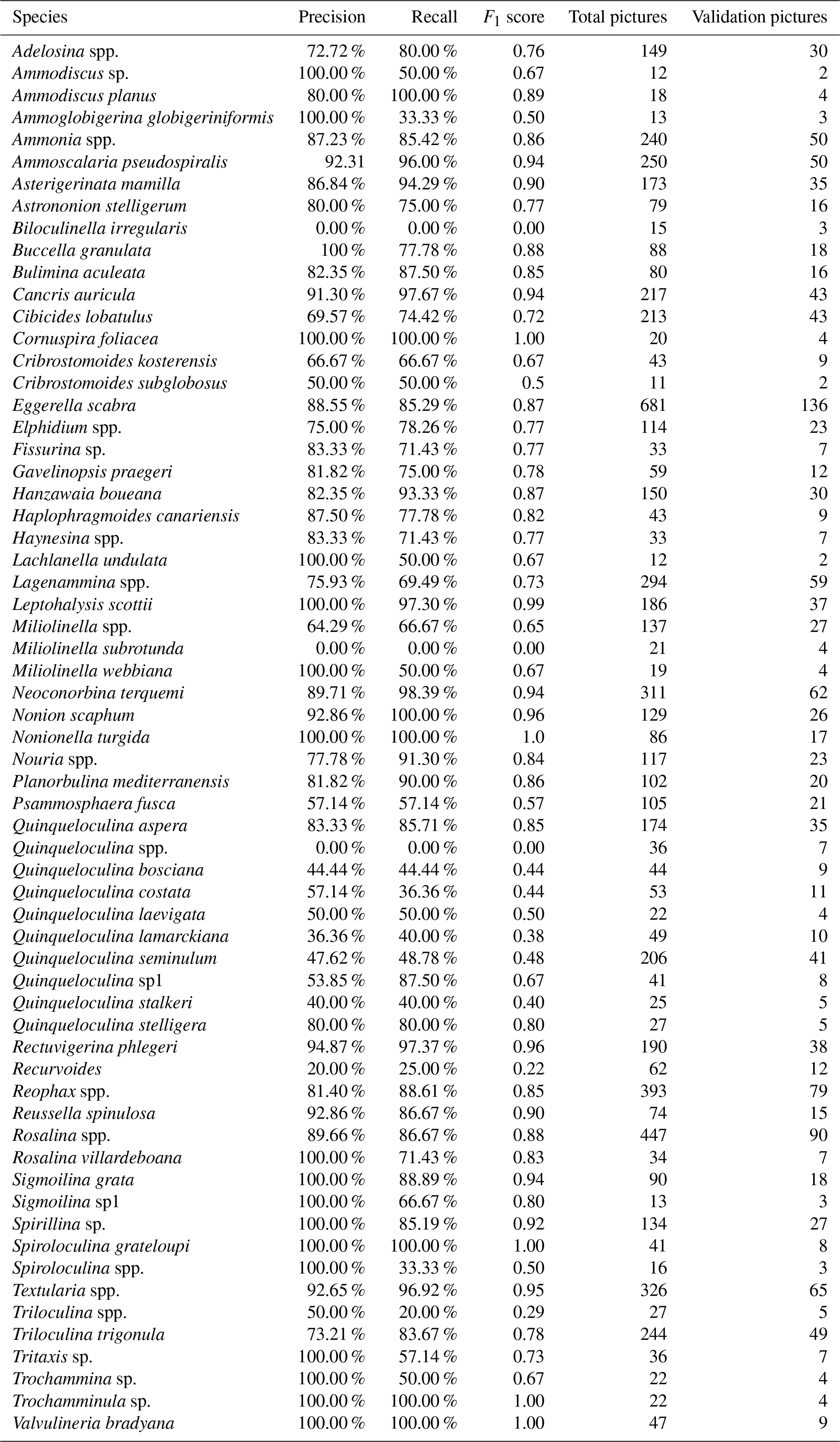
Table G1 Total abundances of foraminifera species in the Mediterranean test sample distal, 05/14; ^* indicates species used to calculate for the TSI-Med (after Parent et al., 2021).

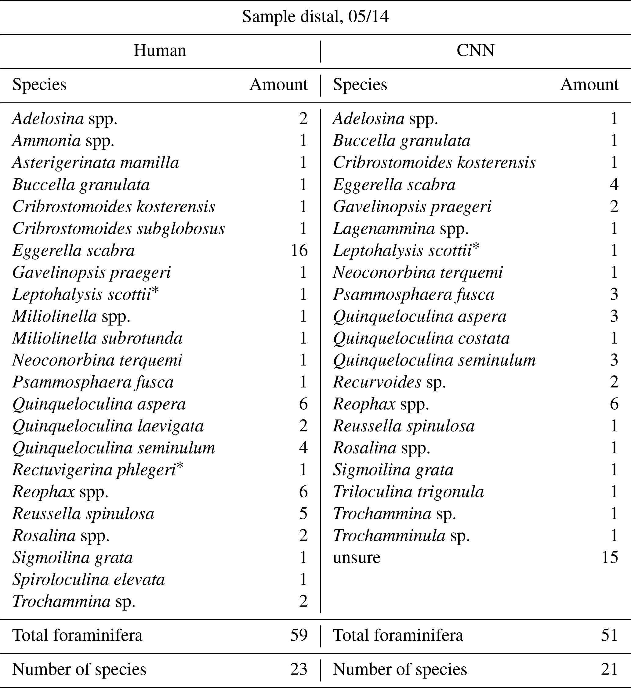
Table G2 Total abundances of foraminifera species in the Mediterranean test sample mid, 05/14; ^* indicates species used to calculate for the TSI-Med (after Parent et al., 2021).

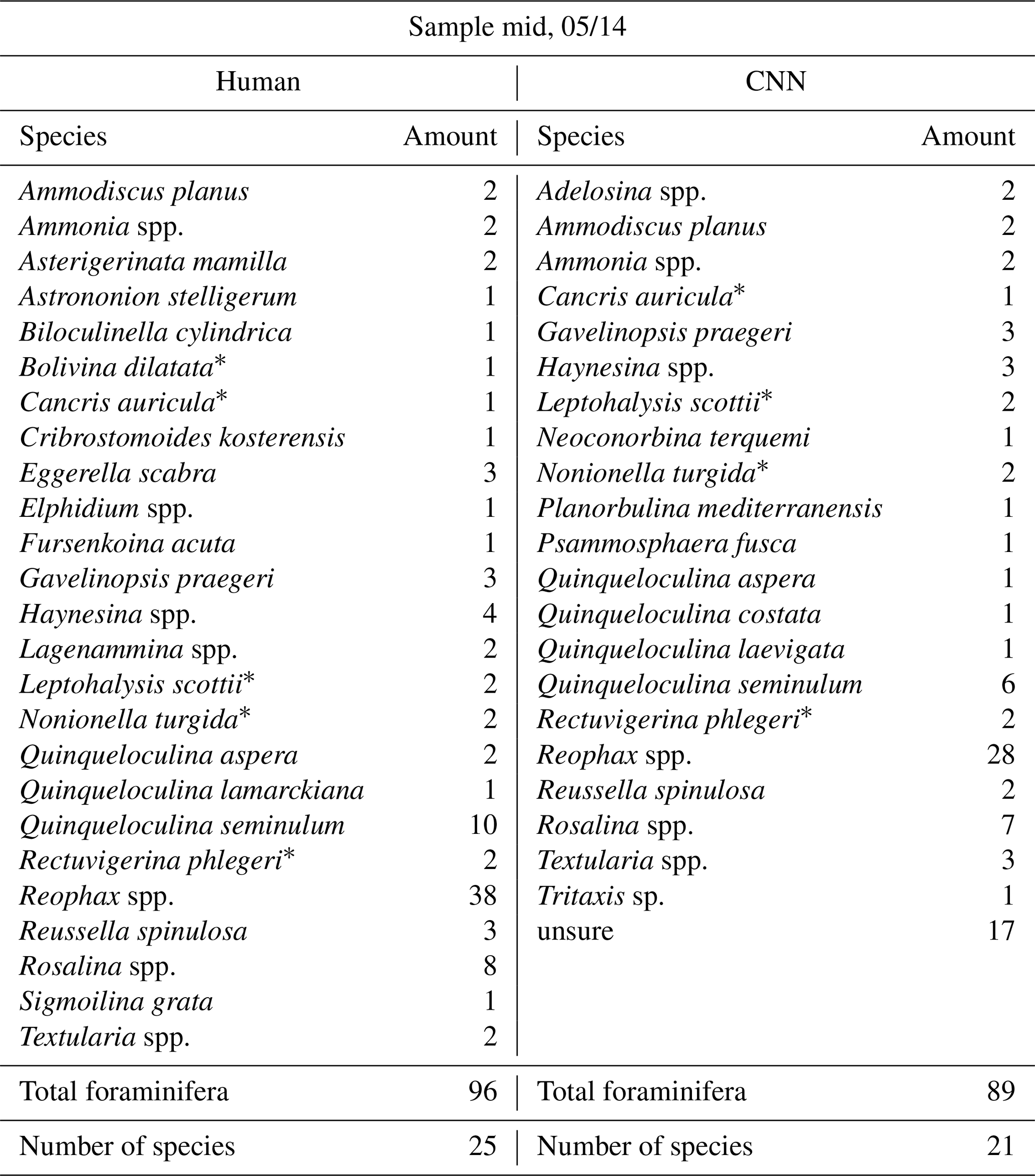
Table G3 Total abundances of foraminifera species in the Mediterranean test sample mid, 09/14; ^* indicates species used to calculate for the TSI-Med (after Parent et al., 2021).

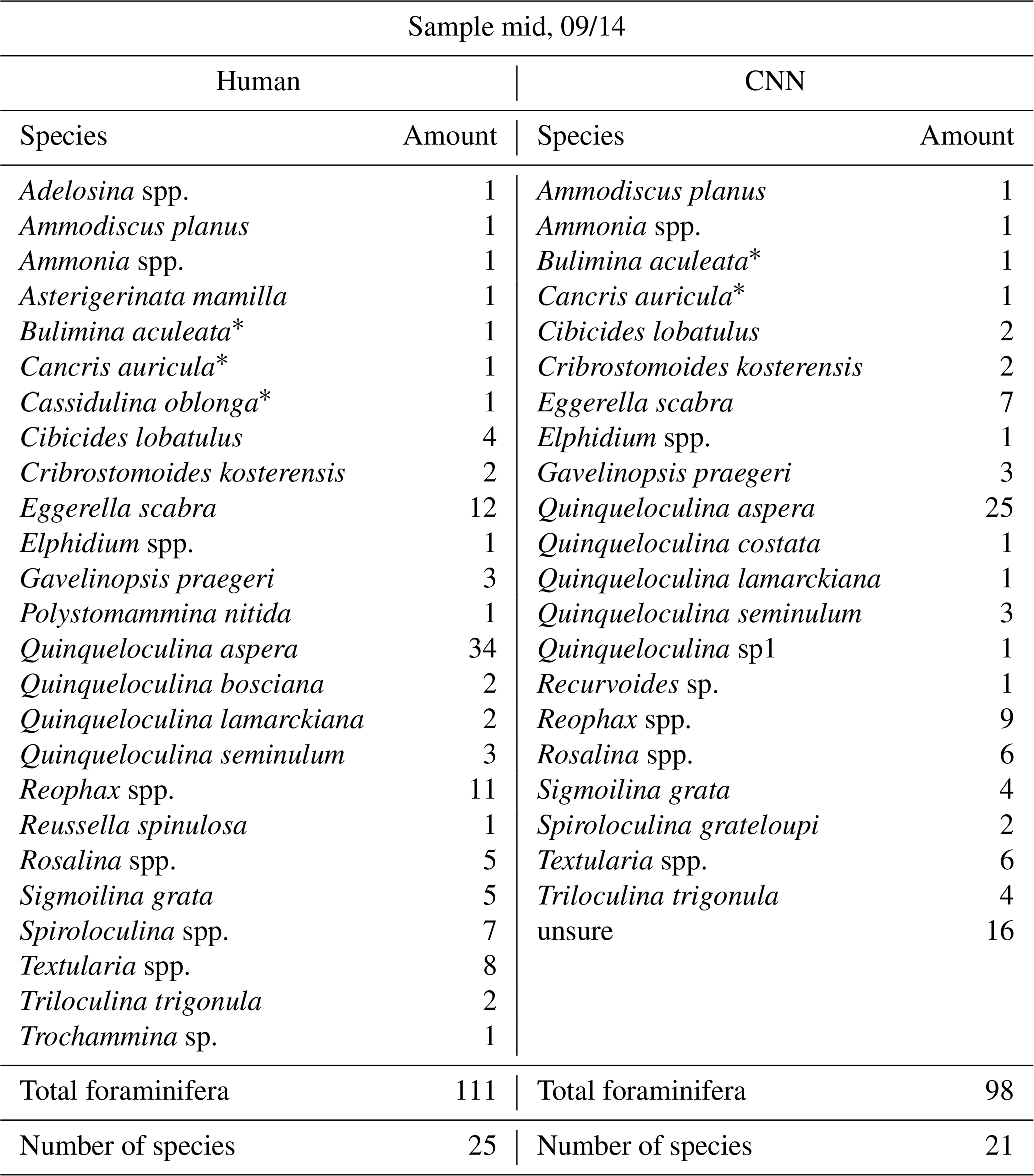
Table G4 Total abundances of foraminifera species in the Mediterranean test sample proximal, 05/14; ^* indicates species used to calculate for the TSI-Med (after Parent et al., 2021).

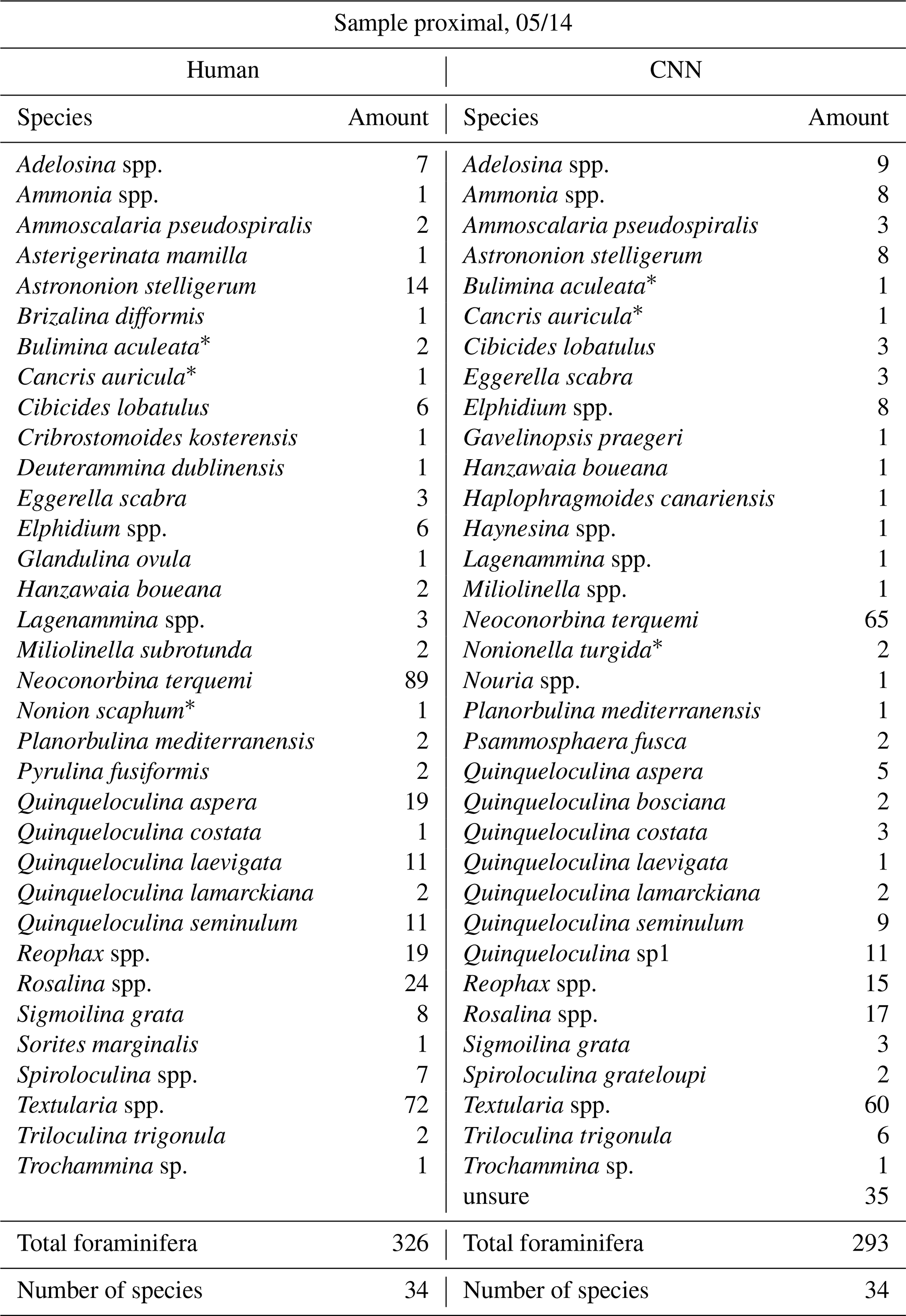
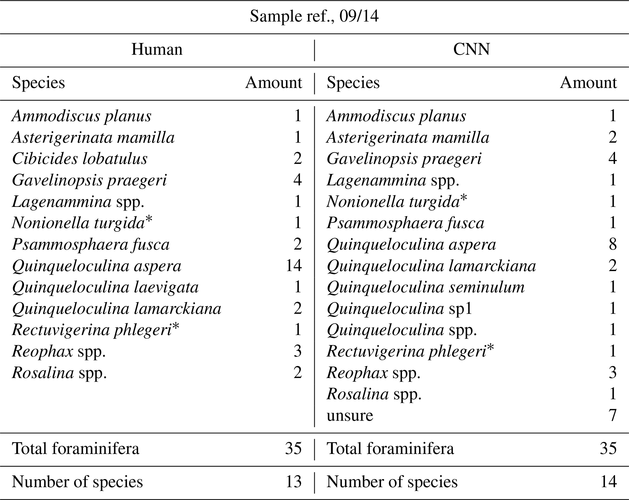
Table G5 Total abundances of foraminifera species in the Mediterranean test sample ref., 05/14; ^* indicates species used to calculate for the TSI-Med (after Parent et al., 2021).

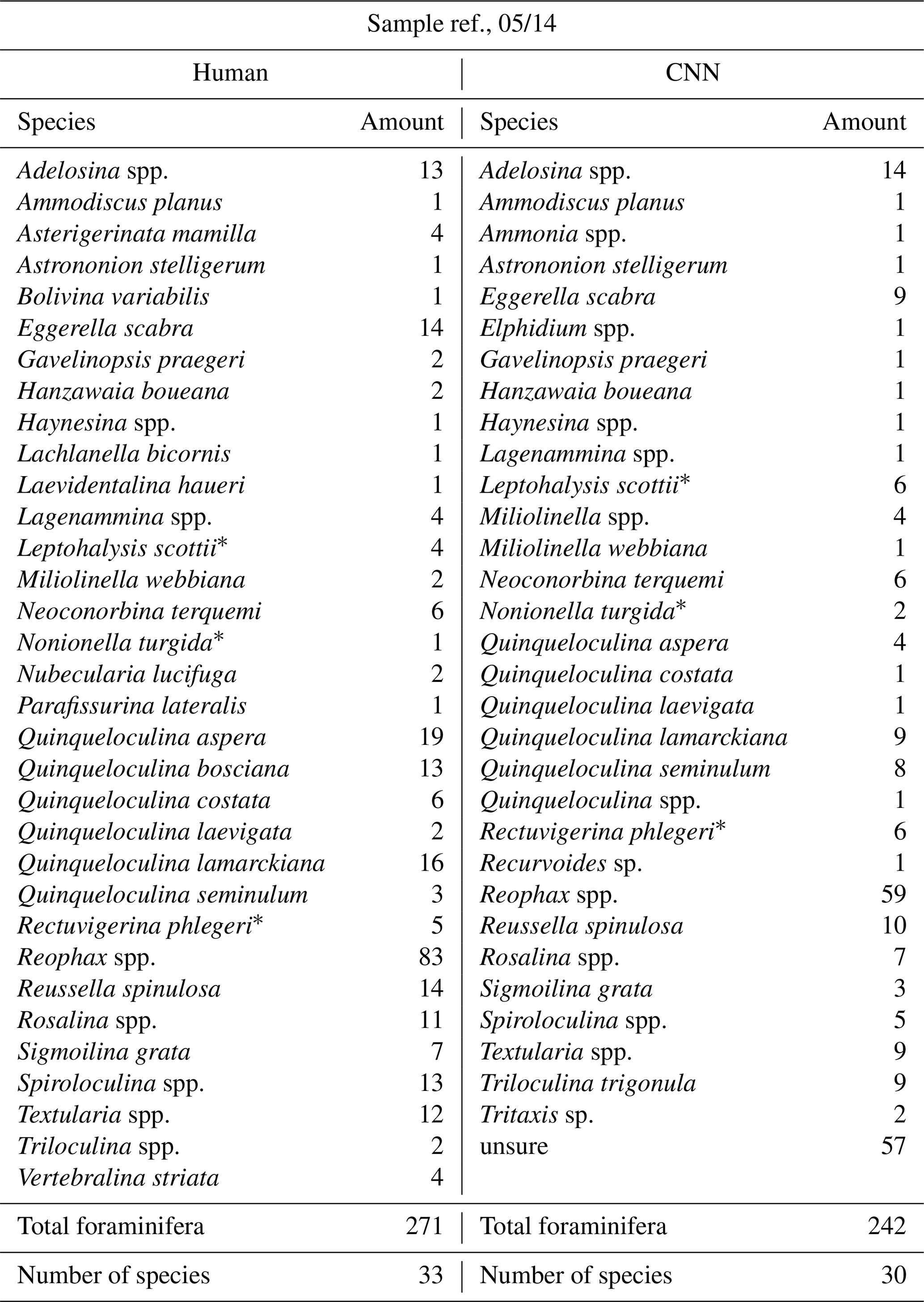
Table G6 Total abundances of foraminifera species in the Mediterranean test sample ref., 09/14; ^* indicates species used to calculate for the TSI-Med (after Parent et al., 2021).