Does Furcatolithus akropodus have two morphotypes useful for biostratigraphic purposes?

The genus Furcatolithus is derived from Sphenolithus; its rapid biological evolution and high diversity make its species excellent markers. This study aims to investigate the distribution of two morphotypes of Furcatolithus akropodus in three ocean basins: the equatorial Pacific Ocean (IODP Hole U1333A), the equatorial Indian Ocean (ODP Hole 711A), and the South Atlantic Ocean (ODP Hole 1265A). The two morphotypes differ by the presence or absence of a midline or groove on the bifid spine, visible under a light microscope, which determines different extinction patterns. Following the approach outlined in previous work, we initially named the form without a line or groove (morphotype A) and the form with a line or groove (morphotype B). To classify the specimens of the species under study, the identification criteria proposed by Howe (2021) were followed. Ultrastructural analysis by scanning electron microscopy (SEM) suggests that morphotype A presents a bifurcation of the bifid spine, probably lateral to morphotype B, in which a central groove or line of the bifid spine is clearly visible, starting from its base and extending to its apex. At the biostratigraphic level, in all three analysed holes, a simultaneous lowest occurrence (LO) of the morphotypes is observed (located at the base of the CNO1 zone), while the highest occurrence (HO) of F. akropodus B precedes that of F. akropodus A, both located in the CNO3 zone. The highest occurrence of F. akropodus A appears to be contemporaneous with the lowest occurrence of F. distentus (base of CNO4 zone). The biostratigraphic order of events resulting from the three holes suggests the biostratigraphic potential of F. akropodus at mid- and low latitudes. The original description, different morphology, and different biostratigraphic distribution allow us to designate F. akropodus A as F. akropodus sinsu strictu and F. akropodus B as F. xiphopodus sp. nov.

1 Introduction

The family Sphenolithaceae is composed of heterococcoliths belonging to the order Discoasterales (Howe, 2021). The genus Sphenolithus originated in the upper Danian (upper Paleocene), probably from the genus Diantholitha. The evolutionary transition involved adding element cycles beyond the single distal cycle present in Diantholitha (Aubry et al., 2011). The oldest known species is Sphenolithus primus (Perch-Nielsen, 1971a). Throughout its evolution, Sphenolithus has maintained a conserved fundamental structure consisting of four main components (Howe, 2021): (1) proximal element cycle (the base of the nannofossil), (2) cycle of lower lateral elements (above the proximal cycle), (3) cycle of upper lateral elements (between the lower cycle and the apical structure), and (4) apical structure (may be composed of a single element, if monocrystalline, or multiple cycles of elements, if composite). During the evolutionary transition from Sphenolithus to Furcatolithus, basal elements progressively decrease in number. In particular Sphenolithus furcatolithoides is considered the transitional taxon between sphenoliths and furcatoliths. The genus Furcatolithus is characterised by the same proximal element cycle present in the genus Sphenolithus but with the loss of the other basal elements. The prominent point is not considered homologous to the apical spine of the sphenoliths (Howe, 2021). The genus Furcatolithus evolved from Sphenolithus during the middle Eocene (Howe, 2021). In the lineage of S. kempii, the upper lateral cycle underwent progressive changes: it grew vertically, and the number of its elements was reduced to two, forming what is called a bifid spine. Definitely, the transition from Sphenolithus to Furcatolithus occurred with the loss of the lower lateral cycle and the apical structure (Howe, 2021). F. cuniculus is considered the oldest species in the genus, descending directly from S. labradorensis through the loss of the lower lateral cycle (Howe, 2021). Notice that S. labradorensis (Firth, 1989; Howe, 2021) and S. strigosus (Bown and Dunkley Jones, 2006) represent the same taxonomic concept, according to Young (2021) (NannoTax). Howe (2021) reports that S. runus is also a synonym of S. labradorensis; furthermore, it has also been considered a possible synonym of S. strigosus and has been related to the S. kempii group (e.g. Bown and Dunkley Jones, 2006; Aubry, 2021).

Unlike Sphenolithus, Furcatolithus species have only two components: the proximal cycle and the bifid spine (Howe, 2021); the latter has been defined as a duo-crystalline spine by Bown and Dunkley Jones (2012) and Bergen et al. (2017). The evolutionary history of the genus Sphenolithus ends in the lower Pliocene (Zanclean) with S. moriformis (S. primus group) (e.g. Bergen et al., 2017), while that of Furcatolithus ends in the lower Miocene (Aquitanian) with F. umbrellus (a species with a greatly reduced or absent bifid spine) (Howe, 2021). The evolution of the genus has previously been discussed by Blaj et al. (2010), Bergen et al. (2017), and Aubry (2021). The last amended diagnosis is from Howe (2021), which is as follows: `

Conical coccoliths with a proximal element cycle of radially arranged elements. Above the proximal element cycle, there is usually a vertically split bifid spine, composed of two vertical elements. The two elements of the bifid spine often bear thin extensions that extend distally and laterally. No lower lateral element cycle, or apical structure (apical cycle or spine), as seen in species of the genus Sphenolithus, is ever present.

The genus Furcatolithus includes 17 species, divided into 3 morphological groups: F. predistentus gr. (Bown and Dunkley Jones, 2012), F. ciperoensis  r. (Bergen et al., 2017), and F. triangularis gr. (Aubry, 2014). The species under consideration is F. akropodus, first described by de Kaenel and Villa (1996) (see Sphenolithus akropodus) while investigating sediments from the Iberian Margin. The same authors identified taxon variability characterised by specimens with a bifid spine that lacks an extinction groove or line and others with one. More recently, Viganó et al. (2023) suggested the presence of two morphotypes at ODP Hole 756C.

A plexus of late Eocene to Oligocene spinose sphenoliths have been widely used in biostratigraphy. Variability, homeomorphic trends, and the occurrence of intergradational forms have hindered their use as marker species and have been the focus of considerable discussion (e.g. Moran and Watkins, 1988; Olafsson and Villa, 1992; Blaj et al., 2010).

The present work aimed to study the optical differences under polarised light between these two morphotypes and their ultrastructure under a scanning electron microscope (SEM) and, finally, to investigate the distribution of these morphotypes to assess whether they can be used to implement the biostratigraphy of the lower Oligocene in low latitudes.

2 Materials and methods

The data used in this study are from our database (Table S1 in the Supplement). In a total assemblage of 500 counted fossils (approximately 5 fields of view (FOVs)), we identified all iso-oriented specimens of Furcatolithus akropodus and distinguished and assessed the relative abundances of the two morphotypes. The biostratigraphic assignment of the samples studied was determined using the main markers of the CNO1–CNO4 interval (C. subdistichus, E. formosa, R. umbilicus, F. distentus) (Agnini et al., 2014). The selected holes are IODP U1333A (Equatorial Pacific Ocean), ODP 711A (Equatorial Indian Ocean), and ODP 1265A (South Atlantic Ocean) (Fig. 1).

Figure 1 Map of current hole locations obtained using R and the “rgplates” and “sf” packages. In parentheses: longitude and latitude, respectively. Current coordinates were obtained from ODP/IODP expedition volumes.

A different number of smear slides (Bown and Young, 1998) were analysed in relation to the sedimentation rates, preservation, and core recovery using Zeiss AxioSkop 2 in phase contrast and crossed nicol mods. We analysed 37 samples at ODP Hole 711A (from 126.050 to 143.550 mbsf), 40 at ODP Hole 1265A (from 147.25 to 158.01 m CSF-A), and 27 at ODP Hole U1333A (from 79.450 to 103.150 m CSF-A), with a resolution between approximately 100 and 10 cm.

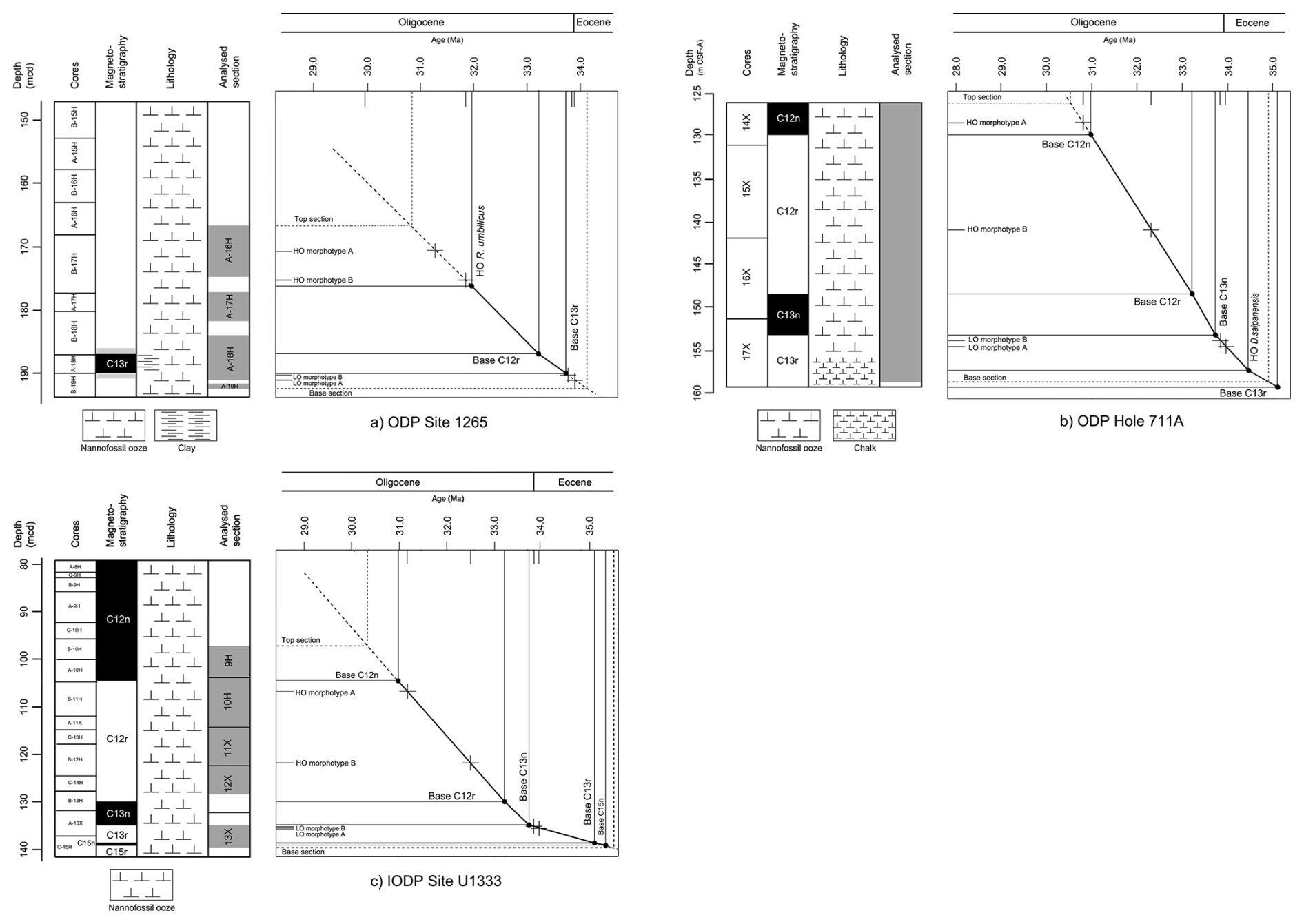
Figure 2 Age–depth models of (a) ODP Site 1265, (b) ODP Hole 711A, and (c) IODP Site U1333 constructed on the basis of reliable magnetic and biological tie points for the calibration of biohorizons located between them. The age of the Chron tops is derived from Speijer et al. (2020) in GTS2020 (Gradstein et al., 2020), as is that of the primary calcareous nannofossil bioevents. The Chron tops were extrapolated from Savian et al. (2013) for ODP Hole 711A, from Zachos et al. (2004) for ODP Site 1265, and from Westerhold et al. (2014) for IODP Site U1333. The dotted line indicates samples whose age has been extrapolated. The black points represent the tie points of the age–depth models.

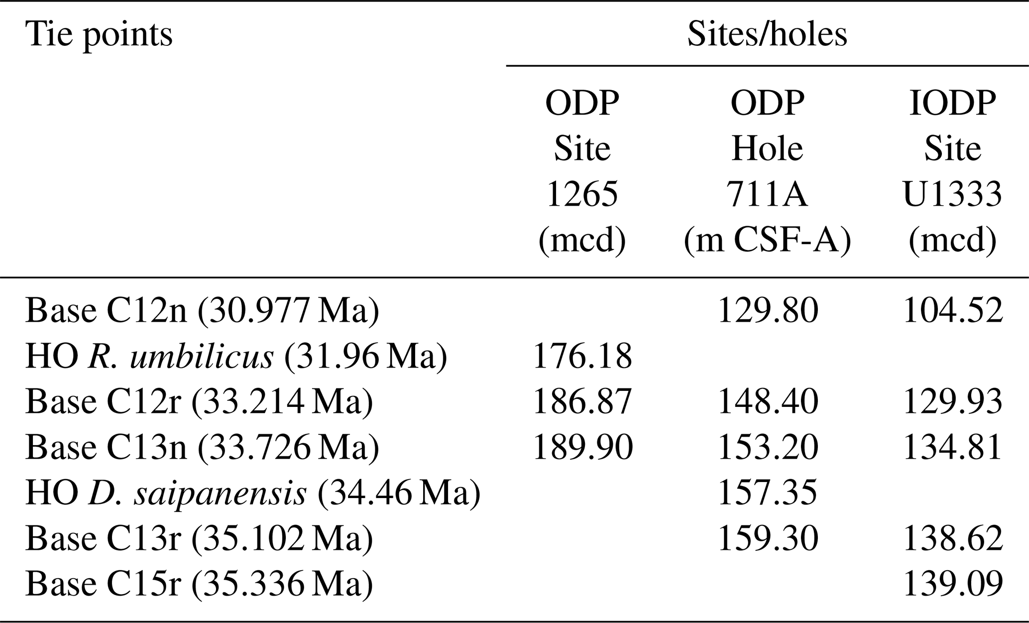
Where possible, we chose the latter value to be close to the crucial intervals of highest occurrence/lowest occurrence of the markers (primary bioevents) and the target species (additional bioevent). We determined preservation using the Bown and Young (1998) method, with categories of poor (P), moderate (M), good (G), and excellent (X), and reported it on a range chart. In the sedimentary sequence covered by this study, the preservation is generally good or good to moderate (Table S1). We then converted the FOV values of the target species (biostratigraphic markers and morphotypes considered) to square millimetres to obtain a useful estimate for biostratigraphic purposes. Subsequently, a SEM analysis was conducted to see whether the differences in morphotypes observed under polarised light could be linked to differences in ultrastructure. To link the specimen viewed under the optical microscope to the one observed under the SEM, we applied the Moshkovitz method (Moshkovitz, 1978). The age–depth models used (Fig. 2a–c) include the tie points reported in Table 1. We calibrated all of these to the most recent geological timescale, GTS2020 (Speijer et al., 2020, in Gradstein et al., 2020). The biostratigraphic interpretations of the holes investigated (711A, 1265A, and U1333A) are based on the biostratigraphic schemes of Martini (1971), Okada and Bukry (1980), and Agnini et al. (2014).

Table 1 Tie points used to construct age–depth models in the studied sections. See Fig. 2 caption for references.

3 Results and discussion

To correctly classify the species, the qualitative approach outlined by Howe (2021) was followed, which highlights that relationships among the median axis/top of the proximal cycle angle, the height of the bifid spine, and the % of the total height of the proximal cycle should be considered. The Furcatolithus species found in the interval under consideration are F. tribolosus, F. predistentus, F. peartie, F. distentus, and F. akropodus, all of which can be clearly distinguished based on the respective parameters listed above. Other species whose range also extends into the Oligocene (Howe, 2021) – F. celsus, F. cuniculus, F. tawfikii, and F. bulbulus – have not been found, perhaps due to their rarity and/or fragility. Observing the two morphotypes of F. akropodus under polarised light, a different extinction pattern can be seen compared to morphotype B (Fig. 3a–d), first described by de Kaenel and Villa (1996) (variants of the same species) and also highlighted by Howe (2021) and Viganò et al. (2023), who hypothesise the existence of these two morphotypes. In detail, it may be noted that morphotype A is completely extinct when placed with the polarising axis parallel to the bifid spine (∼0°), except for nannofossils not perfectly parallel to the horizontal plane, where total/partial birefringence of the proximal element cycle can be observed. At ∼20–25°, half of the proximal element cycle appears birefringent (to the left when rotated clockwise and vice versa when rotated anticlockwise), and the other half is extinct. At ∼45°, it is completely birefringent (Fig. 3a and c; Plate 1, figs. 1–12). Observing morphotype B (which presents an extinction groove or line) at ∼0°, it shows partial birefringence. When the nannofossil is rotated ∼20–25° anti-clockwise, the left side of the bifid spine and the left side of the proximal element cycle light up, whilst the right side of these elements goes extinct; the opposite occurs when rotated clockwise. At ∼45°, it is fully illuminated (Fig. 3b and d; Plate 1 – figs. 13–24), while Howe (2021) states that at 45°, the birefringence of the bifid spine is partial.

Figure 3 Conceptual diagram of how morphotype F. akropodus A (a) and morphotype F. akropodus B (b) appear under polarised light. (c) Polarised light extinction pattern of morphotype A and (d) of morphotype B by varying the inclination of the bifid spine from ∼0° (polarising axis parallel to the bifid spine). Colours are only conceptual.

Plate 1 Light microscope (LM) microphotographs of selected Furcatolithus akropodus from ODP Holes 1265A, 711A and IODP Hole U1333A, all specimens at 1250× magnification. 1. Furcatolithus akropodus A, crossed nicols, ∼0°, 1265A-18-1, 140–141; 2. Furcatolithus akropodus A, crossed nicols, ∼25°, 1265A-18-1, 140–141; 3. Furcatolithus akropodus A, crossed nicols, ∼45°, 1265A-18-1, 140–141; 4. Furcatolithus akropodus A, gypsum lent, ∼0°, 1265A-18-1, 140–141; 5. Furcatolithus akropodus A, crossed nicols, ∼0°, 711A-15-6, 55–56; 6. Furcatolithus akropodus A, crossed nicols, ∼25°, 711A-15-6, 55–56; 7. Furcatolithus akropodus A, crossed nicols, ∼45°, 711A-15-6, 55–56; 8. Furcatolithus akropodus A, gypsum lent, ∼0°, 711A-15-6, 55–56; 9. Furcatolithus akropodus A, crossed nicols, ∼0°, U1333A-12-3, 130–131; 10. Furcatolithus akropodus A, crossed nicols, ∼25°, U1333A-12-3, 130–131; 11. Furcatolithus akropodus A, crossed nicols, ∼45°, U1333A-12-3, 120–121; 12. Furcatolithus akropodus A, gypsum lent, ∼0°, U1333A-12-3, 130–131; 13. Furcatolithus akropodus B, crossed nicols, ∼0°, 1265A-18-1, 140–141; 14. Furcatolithus akropodus B, crossed nicols, ∼25°, 1265A-18-1, 140–141; 15. Furcatolithus akropodus B, crossed nicols, ∼45°, 1265A-18-1, 140–141; 16. Furcatolithus akropodus B, gypsum lent, ∼0°, 1265A-18-1, 140–141; 17. Furcatolithus akropodus B, crossed nicols, ∼0°, 711A-15-6, 55–56; 18. Furcatolithus akropodus B, crossed nicols, ∼25°, 711A-15-6, 55–56; 19. Furcatolithus akropodus B, crossed nicols, ∼45°, 711A-15-6, 55–56; 20. Furcatolithus akropodus B, gypsum lent, ∼0°, 711A-15-6, 55–56; 21. Furcatolithus akropodus B, crossed nicols, ∼0°, U1333A-12-4, 140–141; 22. Furcatolithus akropodus B, crossed nicols, ∼25°, U1333A-12-4, 140–141; 23. Furcatolithus akropodus B, crossed nicols, ∼45°, U1333A-12-4, 140–141; 24. Furcatolithus akropodus B, gypsum lent, ∼0°, U1333A-12-4, 140–141.

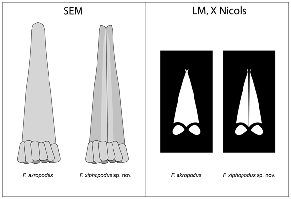
The SEM ultrastructure analysis (Plate 2) confirms the structure also highlighted by Perch-Nielsen (1977), in which the bifid spine is like an elliptical-based cone “embedded” in a cycle of radial crystalline elements. It appears that morphotype A has a lateral bifurcation of the bifid spine, whereas in B it is central, branching from the base of the bifid spine and extending to its apex. This observation is consistent with evidence from the polarised-light behaviour (Plate 1).

Plate 2 SEM microphotographs of selected calcareous nannofossils from ODP Hole 711A and IODP Hole U1333A. 1. Furcatolihtus akropodus B, 8000×, U1333A-12-4, 130–131; 2. Furcatolihtus akropodus B, 13 000×, U1333A-12-4, 130–131; 3. Furcatolihtus akropodus B, 13 000×, U1333A-12-4, 130–131; 4. Furcatolihtus akropodus B, 16 000×, 711A-15-6, 15–16; 5. Furcatolihtus akropodus B, 16 000×, U1333A-12-4, 130–131; 6. Furcatolihtus akropodus A, 15 000×, U1333A-12-4, 130–131; 7. Furcatolithus akropodus A, 12 000×, U1333A-12-4, 130–131; 8. Furcatolihtus akropodus A, 12 000×, U1333A-12-4, 130–131.

Biostratigraphic analysis revealed a continuous distribution of specimens with limited variation in abundance (Fig. 4). The depth range investigated shows good preservation (G) across all three holes. The biostratigraphic events reported below show a certain synchronicity among the analysed holes, suggesting their potential reliability (Fig. 5, Tables 2 and 3). The slight differences in age between the same events at different holes may be due to different sampling resolutions and differences in age–depth models (Fig. 2). It was not possible to investigate at high resolution the interval between the placement of the lowest occurrence (LO) of F. distentus and highest occurrence (HO) of F. akropodus A at Hole U1333A, hence the only slight difference compared to the other holes (see below). Studying additional holes in other sedimentary settings may shed light on the actual contemporaneity of the bioevents mentioned and verify their reliability. In view of the morphological differences observed between the two morphotypes and the differences identified in their stratigraphic distribution ranges, it is considered appropriate to classify morphotype B, which differs from the original description of F. akropodus, as a new species: Furcatolithus xiphopodus sp. nov. (Fig. 6). Hereafter, morphotype B is referred to by this new name (Appendix B).

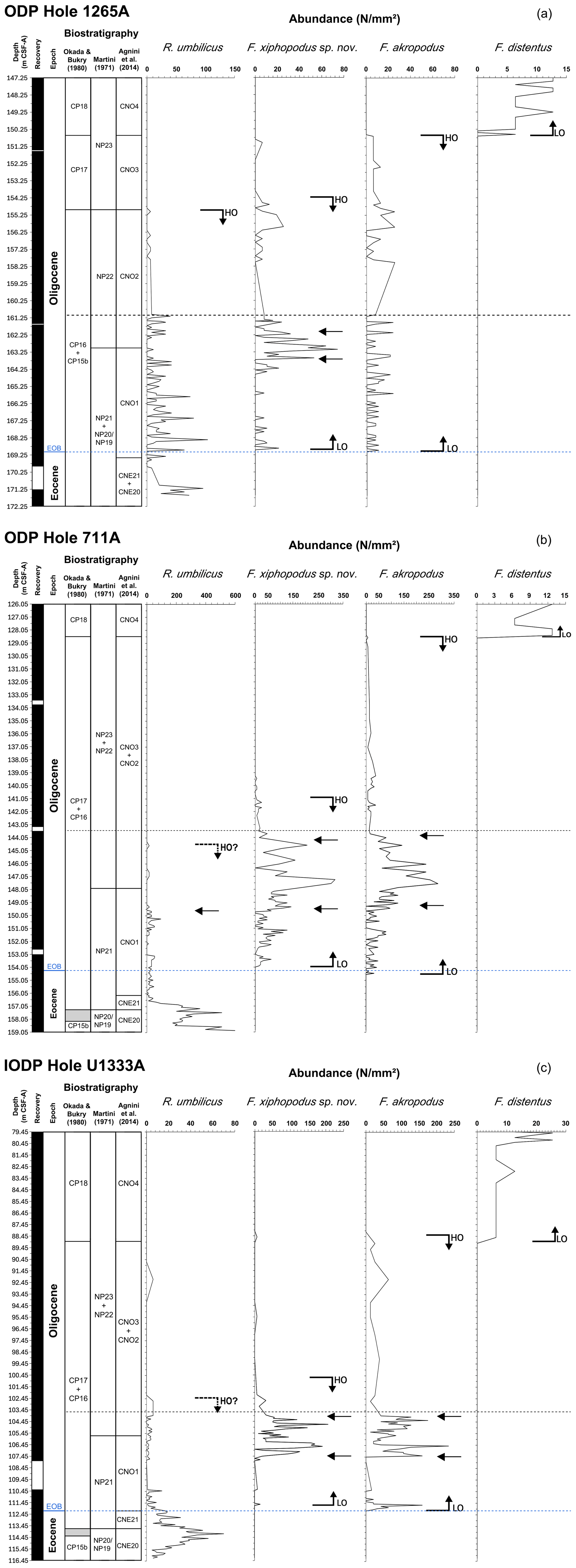
Figure 4 Relative abundance (specimens per square millimetre = N mm⁻²) of primary (F. distentus and R. umbilicus) and additional (Furcatolithus akropodus morphotypes) markers for (a) Hole 1265A, (b) Hole 711A, and (c) Hole U1333A. The position of the biohorizons is plotted against depth (m CSF-A). The Eocene–Oligocene boundary (EOB) is highlighted by a dotted blue line. The dotted black line separates the data yet collected from those of this work. The biozones of Martini (1971), Okada and Bukry (1980), and Agnini et al. (2014) are shown. LO: lowest occurrence; HO: highest occurrence.

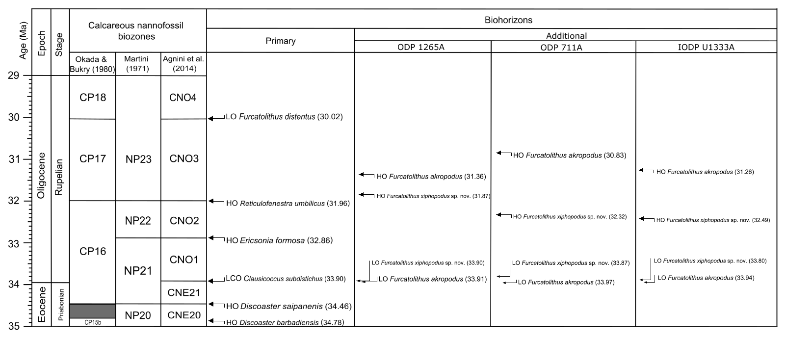
Figure 5 Biozonation diagram of the investigated stratigraphic sequence. The primary (LO F. distentus and HO R. umbilicus) and additional bioevents (LO and HO of F. akropodus morphotypes) discussed are shown. The biozones of Martini (1971), Okada and Bukry (1980), and Agnini et al. (2014) are shown. The age was determined using the most recent timescale (Speijer et al., 2020, in GTS2020, Gradstein et al., 2020). LO: lowest occurrence; HO: highest occurrence.

Figure 6 Key diagnostic morphological characteristics useful for distinguishing F. akropodus s.s. from F. xiphopodus sp. nov.

Table 2 Stratigraphic position of calcareous nannofossil biohorizons in the three analysed holes. Primary bioevents are in bold. The depth of the samples is measured in metres (m) CSF-A. LO: lowest occurrence; HO: highest occurrence.

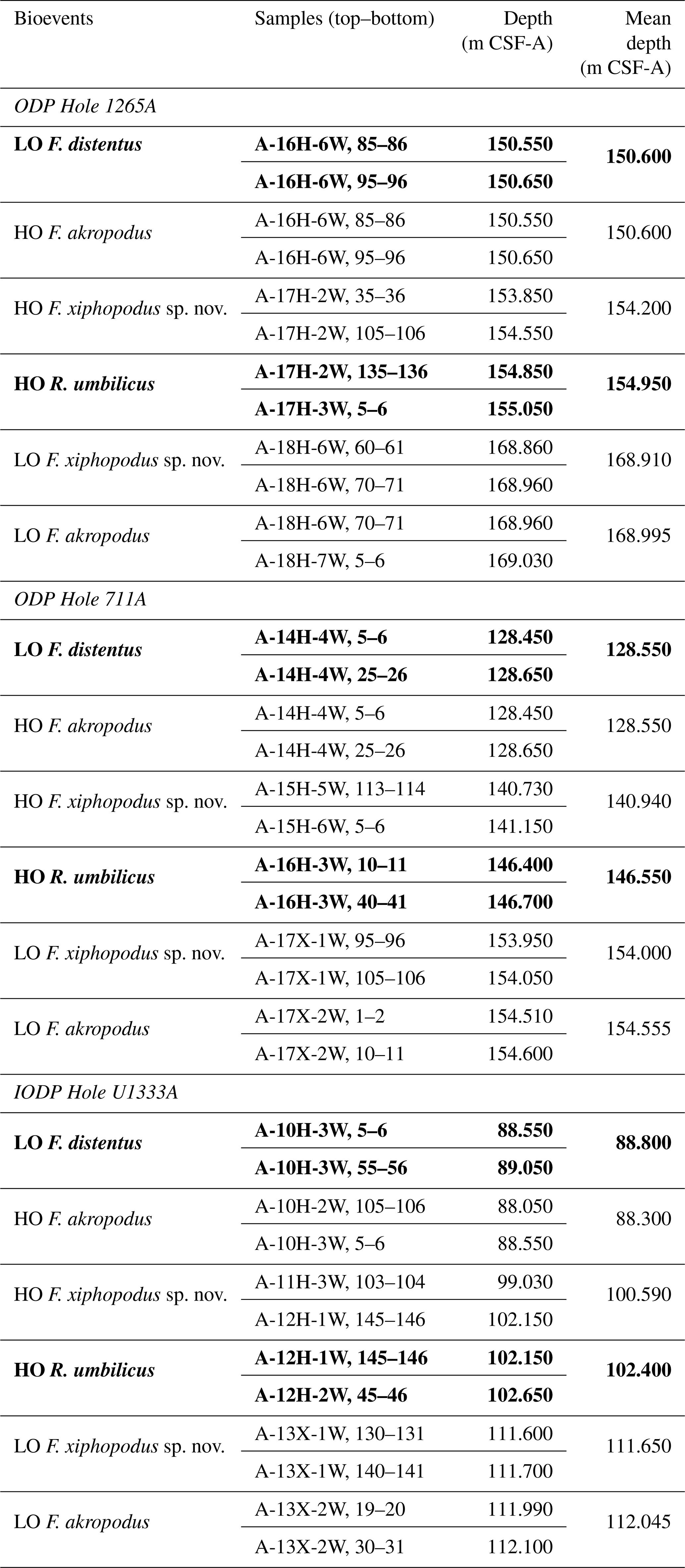
Table 3 Biostratigraphy of calcareous nannofossil biohorizons. The depth of the samples is measured in metres (m) CSF-A. The age was determined using the most recent timescale (Speijer et al., 2020 in GTS2020, Gradstein et al., 2020). LO: lowest occurrence; HO: highest occurrence. Bold type indicates primary bioevents.

LO F. akropodus. The biohorizon is located at the base of the CNO1 zone (or NP21/CP16 zone). It is recorded at 169.995 m CSF-A at Hole 1265A (at ∼33.91 Ma), at 154.555 m CSF-A at Hole 711A (Chron C13r, at ∼33.97 Ma), and at 112.045 m CSF-A at Hole U1333A (at ∼33.94 Ma). Its distribution is continuous, and its occurrence ranges from ∼10 to ∼70–160 N mm⁻² (Fig. 4a–c, Table S1). Following its LO, it reaches peak abundances of ∼260 N mm⁻² at Hole 711A and ∼240 N mm⁻² at Hole U1333A. At Hole 1265A, this pattern is less evident, possibly due to the presence of a data gap between 158.010 and 161.050 m CSF-A (Table S1). After reaching these maximum values, its abundance declines.

LO F. xiphopodus sp. nov. The biohorizon is located at the base of the CNO1 zone (or NP21/CP16 zone). It is recorded at 168.910 m CSF-A at Hole 1265A (at ∼33.90 Ma), at 154.000 m CSF-A at Hole 711A (at ∼33.87 Ma), and at 111.650 m CSF-A at Hole U1333A (at ∼33.80 Ma) It generally appears at low values (see below and Table S1), before peaking (see the interval indicated by the arrows in Fig. 4a–c) and then declining. In detail, it appears with average values of ∼10 N mm⁻² with peaks ∼70 N mm⁻² at Hole 1265A, ∼50 N mm⁻² with peaks ∼370 N mm⁻² at Hole 711A, and ∼10 N mm⁻² with peaks ∼100 N mm⁻² at Hole U1333A (Fig. 4a–c, Table S1). Considering these results, the lowest occurrences of F. akropodus and F. xiphopodus sp. nov. can be assumed to be synchronous for biostratigraphic purposes. The LO of F. akropodus and the LO of F. xiphopodus sp. nov. occur close to the Eocene–Oligocene boundary (EOB), making them potential calcareous nannofossil bioevents for identifying this boundary at low to mid-latitudes.

HO R. umbilicus. The highest occurrence of R. umbilicus marks the base of the CP17 zone (Okada and Bukry, 1980) and the CNO3 zone in Agnini et al. (2014) (Chron C12r, at 32.02 Ma in GTS2012). Some studies report that this taxon is rare and scattered (e.g. Fioroni et al., 2015; Viganò et al., 2023). For Raffi et al. (2016) and Fioroni et al. (2012), it is a reliable biohorizon. At Hole 711A, it is not considered reliable, as at Hole U1333A. It has been recorded only at Hole 1265A, where the biohorizon is located at 154.950 m SF-A. Abundance in all but Hole 1265A is scattered and more limited towards the top of its distribution (Fig. 4a–c; see also the Supplement). At the base of its distribution, R. umbilicus reaches abundances of ∼100 N mm⁻² at Hole 1265A, ∼560 N mm⁻² at Hole 711A, and ∼70 N mm⁻² at Hole U1333A. Its abundance then decreases across the EOB, reaching ∼25, ∼40, and ∼5–10 N mm⁻², respectively. Furthermore, at Hole U1333A, a non-recovery interval is recorded at 107.85–110.31 m CSF-A; it was previously located at 101.17 m CSF-A (Bown and Dunkley Jones, 2012). At Hole 711A, Fioroni et al. (2015) previously located it at 130.86 mbsf and Savian et al. (2013) at 140 mbsf. HO R. umbilicus is used as a tie point in the age–depth model for Hole 1265A (Fig. 2a) because the bioevent is useful given the limited number of tie points. Its age is ∼31.96 Ma (GTS2020). If HO R. umbilicus were located at Hole U1333A, it would be at ∼32.68 Ma, whilst at Hole 711A it would be at ∼32.75 Ma (in both cases in the CNO2 zone), but it could be virtually located earlier, at ∼33.35 Ma (see the arrow in Fig. 4b). These results suggest that the biostratigraphic significance of the HO of R. umbilicus may warrant further investigation, as high-resolution studies such as this one have revealed distributions that make it difficult to place this biohorizon.

HO F. xiphopodus sp. nov. The biohorizon is in the CNO3 zone (early NP23/CP17 zone). The highest occurrence is recorded at 154.200 m CSF-A at Hole 1265A (at ∼31.87 Ma), 140.940 m CSF-A at Hole 711A (∼32.32 Ma), and at 100.590 m CSF-A at Hole U1333A (at ∼32.49 Ma). At the upper end of its distribution, abundance is reduced and slightly discontinuous, as for HO F. akropodus, with values ∼10 N mm⁻² (Fig. 4a–c; see also the Supplement). The discrepancy between Hole 711A and Hole U1333A compared with Hole 1265A may stem from an approximate age–depth model based on a limited number of tie points; therefore, further investigations in other oceanic settings could shed more light on its upper distribution.

LO F. distentus. The species marks the beginning of the CP18 zone (Okada and Bukry, 1980); the upper NP23 zone (Martini, 1971); and, in Agnini et al. (2014), the base of the CNO4 zone (Chron C11r). The estimated age in GTS2020 is approximately 30.02 Ma. Its biohorizon is located at 150.600 m CSF-A at Hole 1265A, at 128.550 m CSF-A at Hole 711A, and at 88.800 m CSF-A at Hole U1333A, previously located at 79.500 m CSF-A by Bown and Dunkley Jones (2012). At Hole 711A, Fioroni et al. (2015) did not record it because it was out of range, but Savian et al. (2013) recorded it in the same hole at 125.8 mbsf. Its lowest occurrence coincides with the highest occurrence of F. akropodus. It occurs at low values across all three holes, ranging from ∼6 to 13 N mm⁻² (Fig. 4a–c; see also the Supplement). At Hole U1333A, its HO is slightly above the LO of F. distentus. This may be due to the unavailability of high-resolution data to investigate the interval between the position of the LO of F. distentus and the HO of F. akropodus. This bioevent is older than the ages reported by Agnini et al. (2014): ∼31.36 Ma at Hole 1265A, ∼30.83 Ma at Hole 711A, and ∼31.30 Ma at Hole U1333A. According to Berggren et al. (1995), this taxon has a temporal range of 31.5–33.1 Ma (within Chron C12r). As with the HO of R. umbilicus, these results suggest that its biostratigraphic significance may require further investigation.

HO F. akropodus. The biohorizon is located on the lower limit of the CNO3 zone (NP23/CP17 zone) (Agnini et al., 2014). Its highest occurrence is recorded at 150.600 m CSF-A at Hole 1265A (at ∼31.36 Ma), 128.550 m CSF-A at Hole 711A (at ∼30.83 Ma), and at 88.300 m CSF-A at Hole U1333A (base of CNO4 zone, ∼31.26 Ma). At the upper end of its distribution, abundance is reduced and slightly discontinuous (Fig. 4a–c; see also the Supplement), with values ∼10 N mm⁻². At the mentioned holes, the highest occurrence of F. akropodus has not been recorded previously. No recent studies show the upper limit of its distribution.

4 Conclusions

The two morphotypes of F. akropodus studied show distinct optical properties under polarised light. F. akropodus s.s. (without a median groove or line on the bifid spine) has a different extinction pattern under polarised light than F. xiphopodus sp. nov., which has a groove or line that can be wide. Polarised light analysis of the structure of the morphotypes of this calcareous nannofossil clearly shows divergent extinction/birefringence patterns. Ultrastructural analysis suggests that F. akropodus has a lateral bifurcation of the bifid spine, whereas in F. xiphopodus sp. nov., it is observed centrally and extends from the base to the apex of the spine. This latter consideration aligns well with the evidence of polarised-light behaviour. Regarding biostratigraphy, there is a simultaneous lowest occurrence (LO) of F. akropodus and F. xiphopodus sp. nov. (base of CNO1 zone), while the highest occurrence (HO) of F. xiphopodus sp. nov. (CNO3 zone) precedes that of F. akropodus. The HO F. akropodus occurs with the HO of F. distentus except for IODP Hole U1333A, where its HO is slightly above the LO of F. distentus. This may be due to the unavailability of high-resolution data to investigate the interval between the position of the LO of F. distentus and the HO of F. akropodus.

These results suggest that F. akropodus and F. xiphopodus sp. nov. may serve as bioevents useful at mid–low latitudes. Investigating the two species in other sedimentary settings could help clarify whether these biohorizons are actually reliable, in particular the HO of F. xiphopodus sp. nov. The occurrence of the LO of F. akropodus and F. xiphopodus sp. nov. close to the EOB highlights their potential as calcareous nannofossil bioevents for identifying this boundary at low to mid-latitudes. These results also suggest that the F. distentus and R. umbilicus biohorizons warrant further investigation, as their LO and HO, respectively, differ from published biochronological calibrations, and the high-resolution data revealed scattered or discontinuous abundances of R. umbilicus, making it difficult to place this biohorizon. Furthermore, it may be worth considering other species of Furcatolithus and verifying whether they show similar differences.

Appendix A

Taxonomic list of calcareous nannofossils:

•  

  Furcatolithus akropodus (de Kaenel and Villa, 1996) Howe 2021

•  

  Furcatolithus xiphopodus sp. nov.

•  

  Furcatolithus distentus (Martini, 1965) Howe 2021

•  

  Reticulofenestra umbilicus (Levin, 1965) Martini and Ritzkowski 1968
  

Appendix B

Furcatolithus xiphopodus sp. nov.

Diagnosis: a large species of Furcatolithus with a long bifid spine bearing a groove or net extinction line extending from the base to the apex of the spine and a short proximal element cycle extending laterally to form the basal part.

Description: this Furcatolithus has a short proximal element cycle and a long bifid spine with an extinction groove or line. At ∼0°, it shows partial birefringence of the bifid spine, and the proximal element cycle is extinct. When the specimen is rotated ∼20–25° anti-clockwise, the left side of the bifid spine and the left side of the proximal element cycle light up, whilst the right side of these elements goes extinct. The opposite occurs when rotated clockwise. At ∼45°, it is fully illuminated.

Size: total length: 7–9 µm; proximal element cycle length: 2.5–3.5 µm

Differentiation: F. xiphopodus has comparable measures to F. akropodus but differs from it by its extinction pattern due to the presence of the groove (or extinction line) on the bifid spine and by a lateral bifurcation of the spine of F. akropodus. According to Howe (2021), it is distinguished from other furcatoliths by the proximal cycle percent of total height (∼15 %), a high bifid spine, and a median axis/top of proximal cycle angle of 65–70°. The proximal element cycle is also almost parallel to the long axis, unlike other Furcatolithus. F. xiphopodus differs from large, similar furcatoliths like F. predistentus because this one has a proximal cycle percent of total height of about 10 % and an axis/top of proximal cycle angle of 80–90°. Finally, it is distinguished from F. ciperoensis by a low median axis/top of proximal cycle angle (<50°) and a proximal cycle percent of total height of about 30 %–45 %, greater than F. xiphopodus.

Derivation of name: from Greek hoplite sword xiphos, and podós – “of feet”

•  

  Holotype: Pl. 1, figs. 17–20

•  

  Paratype: Pl. 1, figs. 21–24

Type locality: ODP Hole 711A, Equatorial Indian Ocean

Type level: Oligocene (Rupelian), Sample ODP-711A-15-6, 55–56 (long.: 61.163000; lat.: −2.742700), Zone CNO1

Occurrence: very abundant to rare in early Oligocene sediments from ODP Hole 711A, IODP Hole U1333, and ODP Hole 1265A. The LO of F. xiphopodus is a reliable event that occurs at ∼33.79–33.97 Ma, and it could be considered contemporary with the LO of F. akropodus (∼33.91–33.97 Ma). HO F. xiphopodus occurs between ∼31.87–32.49 Ma. It is observed at ODP Hole 711A, ODP Hole 1265A, and IODP Hole U1333A.

Range: Early Oligocene Zones CNO1 to CNO3