Benthic foraminiferal patchiness – revisited

Many benthic organisms show aggregated distribution patterns due to the spatial heterogeneity of niches or food availability. In particular, high-abundance patches of benthic foraminifera have been reported that extend from centimetres to metres in diameter in salt marshes or shallow waters. The dimensions of spatial variations of shelf or deep-sea foraminiferal abundances have not yet been identified. Therefore, we studied the distribution of Globobulimina turgida dwelling in the 0–3 cm surface sediment at 118 m water depth in the Alsbäck Deep, Gullmar Fjord, Sweden. Standing stock data from 58 randomly replicated samples depicted a log-normal distribution of G. turgida with weak evidence for an aggregated distribution on a decimetre scale. A model simulation with different patch sizes, outlines, and impedances yielded no significant correlation with the observed variability of G. turgida standing stocks. Instead, a perfect match with a random log-normal distribution of population densities was obtained. The data–model comparison revealed that foraminiferal populations in the Gullmar Fjord were not moulded by any underlying spatial structure beyond 10 cm diameter. Log-normal population densities also characterise data from contiguous, gridded, or random sample replicates reported in the literature. Here, a centimetre-scale heterogeneity was found and interpreted to be a result of asexual reproduction events and restricted mobility of juveniles. Standing stocks of G. turgida from the Alsbäck Deep temporal data series from 1994 to 2021 showed two distinct cohorts of samples of either high or low densities. These cohorts are considered to represent two distinct ecological settings: hypoxic and well-ventilated conditions in the Gullmar Fjord. Environmental forcing is therefore considered to impact the population structure of benthic foraminifera rather than their reproduction dynamics.

1 Introduction

The spatial distribution of organisms in their habitats often does not follow a uniform pattern (Gleason, 1920). Aggregated or patchy distribution patterns of higher organisms have been studied in detail in both terrestrial and marine ecosystems (e.g. Brenchley, 1982; Brown, 1984; Legendre and Fortin, 1989; Cole et al., 2000). Restricted motility, limited proliferation of juveniles, social attraction, bio-irrigation by macrofauna, and, more importantly, a heterogenous distribution of food or ecological niches due to a high variety of habitats have been identified as causes of aggregated distributions in marine ecosystems (e.g. Kershaw, 1963; Reise, 1979; Findlay, 1981; Rice and Lambshead, 1994; Buhl-Mortensen et al., 2010). In the deep sea, aggregated distributions have been documented for benthic macrofauna and meiofauna, including metazoans and foraminifera (Hessler and Jumars, 1974; Bernstein et al., 1978; Bernstein and Meador, 1979; Griveaud et al., 2010; McClain et al., 2011; Danovaro et al., 2013; Lejzerowicz et al, 2014). When the substrate is as uniform as a soft-bottom seabed and the benthic organisms of interest are very small, it is challenging to disentangle the patterns and reasons for their spatial structure or lack thereof (e.g. Hasemann and Soltwedel, 2011; Mosch et al., 2012).

Benthic foraminifera are millimetre to sub-millimetre in size and occur in all marine environments. Replicate sampling in early studies revealed high variability in population densities and species' abundances at small spatial scales (Parker and Athearn, 1959; Richter, 1961). This pattern was interpreted to reflect irregularly distributed, transient colonies (Todd and Low, 1961), and sampling schemes for benthic foraminifera were adapted accordingly (Brooks, 1967). As a result, different investigation strategies were pursued to assess the aggregated distribution of benthic foraminifera. For example, contiguous sampling of cubes with an equal size was performed in intertidal environments (e.g. Buzas, 1968; Lehmann, 2000; de Nooijer, 2007). The frequency distribution of population densities obtained from the array was tested against a binominal distribution. If, for instance, a chi-square test rejected the hypothesis, the distribution was considered to be non-homogenous, i.e. aggregated (Buzas, 1968). Subsequent studies used graphical visualisations of population density patterns or scale variance analyses to depict aggregations (Lutze, 1968a; Wefer, 1976; de Chanvallon et al., 2015, 2022). The gathered knowledge from these studies resulted in the model of centimetre-sized patches of foraminiferal abundances that pulsate in time and space due to restricted juvenile mobility (Buzas et al., 2002, 2015). The gathering of juveniles around the parental test after asexual reproduction has been corroborated by live observations, providing support for this model (e.g. Murray, 2012, and references therein).

Foraminiferal patchiness investigations in subtidal waters were pursued with samples taken equally spaced at a decimetre to metre scale along transects or in regular grids (Lynts, 1966; Lutze, 1968a; Schafer, 1971; Hohenegger et al., 1993). Other studies performed repetitive sampling with a grab or corer from a swaying vessel at anchorage or at station (e.g. Brooks, 1967; Haake, 1967), subdivided a large box core into subsamples (e.g. Bernstein et al., 1978; Kaminski, 1985), or investigated adjacent samples from a multiple coring device (e.g. Barras et al., 2010). Higher faunal variations among subsamples from the same box core than between adjacent box cores suggested patchiness on scales of 40 cm or less (Kaminski, 1985). Contour maps depicted confined abundance maxima of metres in diameter (Vangerow, 1977). They were mainly expressed in the absolute abundances of the most frequent species and were consequently related to local food particle enrichments on the sea floor (Lutze, 1968a). Much larger patch sizes of kilometres or more were inferred from species distributions on the continental shelf and in the deep sea (e.g. Heinz et al., 2005; Dorst and Schönfeld, 2013; Stefanoudis et al., 2016). These patterns were related to substrate properties and local variations in food supply or hydrodynamic conditions (Heinz et al., 2004; Schönfeld and Altenbach, 2005; Dorst et al., 2015).

The aim of the present study was to test whether metre-scale or larger spatial variations in foraminiferal population densities prevail in a soft-bottom seabed under calm hydrodynamic conditions or whether patches of a much smaller scale predominate. We used a large population density data set of Globobulimina turgida from the Alsbäck Deep, Gullmar Fjord, Sweden, to test the hypotheses. The species' abundances from precisely located samples were compared with simulated aggregation patterns of various impedances, shape and patch sizes. The abundances were also compared with a temporal data series from the same location, literature data from earlier studies on foraminiferal patchiness, and forced patchy distribution data on insects from a terrestrial ecosystem.

2 Material and methods

2.1 Shipboard operations and sampling

The samples were taken at the Alsbäck Deep in the Gullmar Fjord, Sweden, where the benthic foraminiferal faunas have been investigated since the 1940s (Höglund, 1947; Gustafsson and Nordberg, 2001; Filipsson and Nordberg, 2004; Risgaard-Petersen et al., 2006; Bergstrand, 2012; Koho et al., 2011; Polovodova Asteman and Nordberg, 2013; Polovodova Asteman and Schönfeld, 2016). The samples were taken around the target location at 58^∘19.38^′ N, 11^∘32.74^′ E and 118 m water depth from the R/V Oscar von Sydow on 29 and 31 July 2015. Eight subsequent deployments were performed with a MiniMuc K/MT 410 interface corer on each day (Appendix Table A1), and four samples were collected in each deployment. The vessel compensated for drift during winch operations to keep the wire as vertical as possible. The bottom contact positions of the deployments were recorded with a handheld Garmin Etrex^® GPS. The 50 % circular error probable (CEP) was 4 m during the operations. All deployments touched the seabed in a circle of 54 m diameter around the target location with a probability of 95 % (Fig. 1). The MiniMuc interface corer was equipped with four tubes of 610 mm length and 100 mm inner diameter, which were arranged in a square with a midpoint distance of 21 cm (Kuhn and Dunker, 1994). The cores from each deployment were designated as A through D and treated independently.

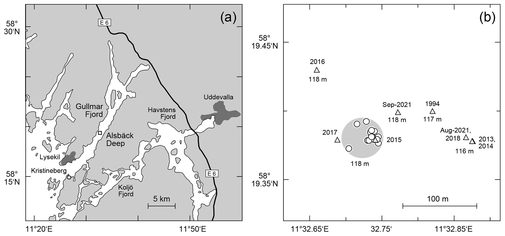
Figure 1 (a) Map of the study area with larger cities (dark grey polygons), the E6 motorway from Gothenburg to Oslo, the location of the Sven Lovén Centre at Kristineberg (circle), and the Alsbäck Deep (square). (b) Detailed map of the sampling locations at the Alsbäck Deep. Circles: replicate samples taken in July 2015. Triangles: samples of the temporal data series taken from 1994 to 2021. Large light-grey circle: area of 95 % probability of replicate samples around the target location. The symbol diameter of the replicate samples indicates ±4 m CEP of the sampling positions. The years of sampling and water depths are given for comparison.

A total of 64 samples were taken around the target location to collect as many viable specimens as possible from the endobenthic foraminiferal species Globobulimina turgida (Bailey, 1851) for a physiological experiment (Woehle et al., 2018; Appendix Table A2). The abundance maximum of this species was confined to the uppermost 3 cm of the surface sediment at the Alsbäck Deep (Risgaard-Petersen et al., 2006). Sampling, sample preparation, and analyses therefore differed from earlier studies of Alsbäck Deep foraminifera (e.g. Bergstrand, 2012; Polovodova Asteman and Nordberg, 2013) and from recommended biomonitoring methods for foraminifera (Schönfeld et al., 2012, 2013).

In brief, the supernatant water of the cores was siphoned off with a TYGON^® hose before sampling. The whole 0–3 cm surface sediment was sliced off with a graduated ring and shuffle spatula used as a cutting plate (Schönfeld et al., 2012, their fig. 2). The sediment slice was dropped down in the upright position into a cylindrical, 500 mL polypropylene (PP) vessel of 112 mm inner diameter. The level of sample fill was marked outside on the vessel with a permanent marker. The samples were then covered with bottom water, transported, and stored at 8 ^∘C.

Additional foraminiferal samples were taken from the 0–3 cm surface sediment at the Alsbäck Deep during the summer in 2013, 2014, 2016 through 2018, and 2021 (Appendix Table A3). The 2013 sample was taken with a multicorer, and the 2016 to 2021 samples were taken with a double-spade Ekman-type box corer. Directly after the box core came on deck, a push core was taken from the middle of the box to retrieve the top 3 cm of the sediment as undisturbed as possible. Literature data on G. turgida population densities at the Alsbäck Deep in 1994, 2005, and 2011 were also considered to establish a temporal data series (Gustafsson and Nordberg, 2001; Risgaard-Petersen et al., 2006; Bergstrand, 2012).

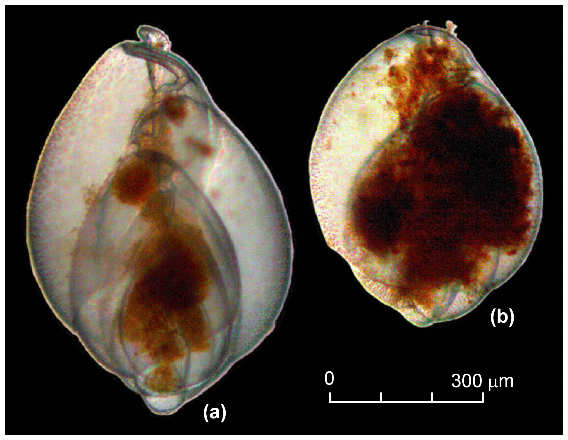
Figure 2 Bright field images of colouration and cytoplasm fill of living G. turgida individuals: (a) with a low amount of cytoplasm concentrated around the central spindle and (b) with chambers filled with cytoplasm.

2.2 Sample preparation

The replicate samples were gently washed through stacked sieves of 2000 and 125 µm with Gullmar Fjord “deep water” from the tap in the Intagshallen laboratory, Sven Lovén Centre Kristineberg, Sweden, a few hours after core recovery on the same day. The mesh size of 125 µm was chosen because it has proven to be the best compromise between time effort necessary for picking the samples and completeness in capturing the species inventory (Schönfeld et al., 2012, 2013). We screened the size fraction 63–125 µm of sample OVS290715-5D. Only small-sized Textularia earlandi and no other species were found. Bolivina pseudopunctata, Stainforthia fusiformis, and Epistominella vitrea were found in the >63 µm fraction of other samples. The deep water is pumped from ca. 30 m depth. It had a salinity of 31.8 psu and a temperature of 13.8 ^∘C, thus differing in an acceptable range from the 34.1 psu and 7.2 ^∘C measured in the near-bottom water at the sampling site. The residue >2000 µm containing fragments of polychaeta tubes, plant debris, shells, and other macro-organisms was disposed of. The residue 125–2000 µm was filled in 60 mL Nalgene^® PP beakers and covered with artificial seawater (ASW; Kester et al., 1967) with a salinity of 29.5 psu.

The sample vials were filled with water up to the sample's fill mark level after washing. The volume of the water representing the bulk sample volume was measured in a graduate pitcher with an accuracy of ±5 cm³. The level mark on the sample vials of deployment OVS 290715-8 was not recognisable any more after washing, and their sample volumes could not be determined.

2.3 Picking of foraminifera, vitality assessment, and faunal analyses

The residues were picked wet for living individuals of Globobulimina sp. immediately after washing. All specimens from a sample were collected with featherweight forceps and transferred to a petri dish of 35 mm diameter with sterile ASW for further manipulations. We did not differentiate between G. turgida sensu stricto (s.s.) and G. auriculata morphotypes. Diagnostic morphological characteristics for species discrimination, such as the apical spines and serrated tooth plate of G. turgida s.s. (e.g. Woehle et al., 2018, their fig. 1), were often obscured or not visible under water. Furthermore, the morphotypes were considered to be cospecific at the time of sampling, and the species name G. turgida was given priority (Alve, 2010; Murray and Alve, 2016, and references therein). The specimens were counted, their cytoplasm shape, colour, and internal structures were cross-checked, and their vitality was discussed among the pickers. Organisms were considered viable if they

• had a glossy, transparent, and undamaged test;

• showed a structured infill of dark-yellowish to brown cytoplasm, containing either vacuoles with an infill of different colour or dark-brown minuscule granules;

• presented an infill in more than two connected chambers (Fig. 2) – sometimes the infill was concentrated or tangled around the central spindle with an extension to the aperture, or the infill was concentrated in isolated spots or parts of the chambers of some other specimens; and

• had a film or strings of cytoplasm, presumably pseudopodia firmly sticking to sediment grains, nematodes, or other foraminifera either alive or as empty tests.

Our vitality assessment by visual cytoplasm evaluation was compared with that obtained by the conventional staining method (Lutze and Altenbach, 1991; Murray and Bowser, 2000; Schönfeld, 2012). In particular, all living G. turgida specimens and the remaining residue of sample OVS310715-6A were preserved and stained with a solution of 2 g rose bengal in 98 % ethanol. Sample residue and picked foraminifera were washed with tap water through a 63 µm mesh 2 months after collection. The well-stained foraminifera were wet-picked, sorted by species in Plummer cell slides, fixed with glue, and counted.

The temporal data series samples were also preserved, stained with ethanol–rose bengal, and washed with tap water through stacked 2000 and 125 µm sieves, and the fraction 125–2000 µm was picked and analysed following the same techniques as sample OVS310715-6A. Most of the G. turgida s.s. and G. auriculata morphotypes could be discerned in the temporal data series samples. Their abundances were added for further analyses in order to remain compatible with the replicate sampling data where the morphotypes were not discerned.

2.4 Literature data

Non-contiguous sample series from subtidal environments at Eckernförde Bight and Bottsand lagoon in the Baltic Sea (Lutze, 1968a), as well as from Narragansett Bay, Rhode Island, USA (Brooks, 1967), were considered in the present study for comparison (Supplement 1). Contiguous sample series from intertidal environments of the Loire River estuary (France), Rehoboth Bay (Delaware, USA), and Schobüll (Germany) were considered as well (Buzas, 1968; Lehmann, 2000; de Chanvalon et al., 2015). All these studies reported standing stock data for the most abundant species. The sample numbers were too low or their spatial arrangement was either unknown or unsuitable for an assessment of their spatial heterogeneity with autocorrelation techniques (Legrende and Fortin, 1989; Thrush, 1991). Therefore, the frequency distribution patterns of standing stocks were analysed from the literature data (Perry et al., 2002). The frequency distributions were compared with data obtained in the present study. They were also compared with the frequency distribution of Drosophila simulans Stuartevant (1919) abundances from a mesocosm experiment with decaying nectarines (Supplement 1). Different microclimate treatments generated an expected abundance pattern of confined patches during the experiment. The patches were mirrored by a spatial autocorrelation pattern and displayed by omnidirectional correlograms of Moran's I values (Warren et al., 2006, 2009).

2.5 Data treatment

Population densities of G. turgida were calculated from the bulk sample volumes and numbers of living specimens. The standing stock values are given in individuals per 10 cm³ of the 0–3 cm surface sediment. These were standardised to a mean value of 0 and standard deviation of 1. Population densities of individual species from other studies, in which contiguous, gridded, or replicate samples were used, were also standardised to the mean and standard deviation. The population density data were log-transformed and standardised for comparison with ideal normal distributions.

Statistical tests applied to the data include the Kolmogorov–Smirnov (KS) goodness-of-fit test, Wilcoxon signed-rank test, and Lilliefors test (e.g. Sachs and Hedderich, 2006). The data analyses were performed with the Statistics and Machine Learning Toolbox of the MATLAB^® and PAST programmes, as well as web-based applications (Hammer et al., 2001; Hemmerich, 2018). Log-probability plots were created with KaleidaGraph™ V3.5.

2.6 Model design and operation

A model simulation with different patch sizes, outlines, and impedances, as well as 1000 different random distributions each was executed with MATLAB^® by Giddy Landan (genomic microbiology group, Institute of Microbiology, Kiel University). The following assumptions and simplifications were made: the MiniMuc deployment positions were taken as measured and the CEP was not considered. The orientation of the four-tube array was not random but aligned. The geographical coordinates were converted to Cartesian coordinates with 1^′ latitude equalling 1860 m and 1^′ longitude equalling 975 m. They were rotated counterclockwise by 141.5^∘and horizontally mirrored in order to minimise space and to avoid negative values on the ordinate. The converted deployment positions were centred in a grid of 21×56 m and 0.1 m resolution, which matches the MiniMuc dimension at the lowest resolution.

Patchiness structures were simulated by random selection of focal points and labelling of every point in the sampling area by its distance to the closest focal point. A large range of focal point concentrations was considered, and for each concentration 1000 random patterns were generated. In addition, a log-normal random sample without any spatial structure was created.

Two types of functional relationships between population densities and distance from foci were considered. In the “peaks” regime, the focal point was associated with maximal density and densities decreased with increasing distance from the peak. In the “pits” regime, the focal point was associated with the minimal density and densities increased with distance from the pit. The “peaks” scenario produces local aggregations, whereas the “pits” scenario produces local depletions. In both regimes, the optimal functional dependency was estimated by regression of the empirical distribution function of the actual population densities on the distribution of simulated distances from all 1000 random patterns created for one focal concentration.

Simulated population densities were calculated by applying the regression equation to every sample point in each of the 1000 random patterns. For each of those model runs, the distribution of simulated densities to the actual densities were compared by using the two-sided two-sample KS test (e.g. Sokal and Rohlf, 1995). The 1000 p values were visualised as cumulative frequency distributions. In a satisfactory model, the simulations resemble the observations and should theoretically produce a uniform distribution of p values ranging from 0 to 1; i.e. a plot of sorted p values will lie on the diagonal. In addition, the expected mean and median of the p values will be 0.5. The latter equality was tested by using the Wilcoxon test.

3 Results

3.1 Vitality assessment

Preservation of the 68 picked G. turgida specimens from sample OVS310715-6A was good, and the infill of 66 individuals was raspberry red after rose bengal staining. Two specimens showed a dull brownish colouration. They also showed spots of unstained, fine-grained sediment particles in the ultimate chamber and in the aperture, providing evidence that they were probably not alive at the time of sampling. A total of 10 more stained G. turgida were found in the remaining residue from, 2 of which were the same size as the previously picked specimens and brightly stained throughout the test. Eight specimens were very small and showed a variable staining pattern. These figures revealed that 87 % of all living G. turgida in this sample were recognised during sample screening after washing based on their visual cytoplasm characteristics. This recognition rate was similar to an earlier methodological study (90 %; Schönfeld et al., 2013), and hence it is considered sufficiently reliable for the assessment of G. turgida communities.

3.2 Community parameters of G. turgida

The living, rose-bengal-stained foraminiferal fauna at the Alsbäck Deep comprised 27 different species in the summer of 2015. Globobulimina turgida at 6.8 % was the third-ranked species after Nonionella turgida (68.1 %) and Bulimina marginata (8.4 %). Nonionella stella (4.8 %) and Nonionella labradorica (4.7 %) were common in the living fauna as well. Other species were rare with relative abundances not exceeding 1.2 % (Appendix Tables A3, A4). The summer population density of the entire fauna >125 µm was 37.8 living specimens per 10 cm³ in 2015. The density varied between 20.5 and 85.1 specimens per 10 cm³ from 2013 to 2021.

The G. turgida standing stock was 2.6 specimens per 10 cm³ in the living fauna from sample OVS310715-6A. The data from all 2015 replicate samples varied from 0.6 to 5.0 living G. turgida per 10 cm³, on average 2.1±1.1 (1σ value, n=58; Appendix Table A2). The median was 1.8 specimens per 10 cm³, i.e. slightly lower than the mean, indicating a right-skewed data distribution (skewness 0.84) (Fig. 3). The p value of a KS test with Lilliefors modification was 0.014, thus rejecting the hypothesis of a normal distribution. Once the G. turgida standing stock data were log-transformed, the p value was 0.236, indicating a normal distribution at a >0.99 significance level. This indicates a log-normal distribution of G. turgida standing stocks in the 2015 replicate samples.

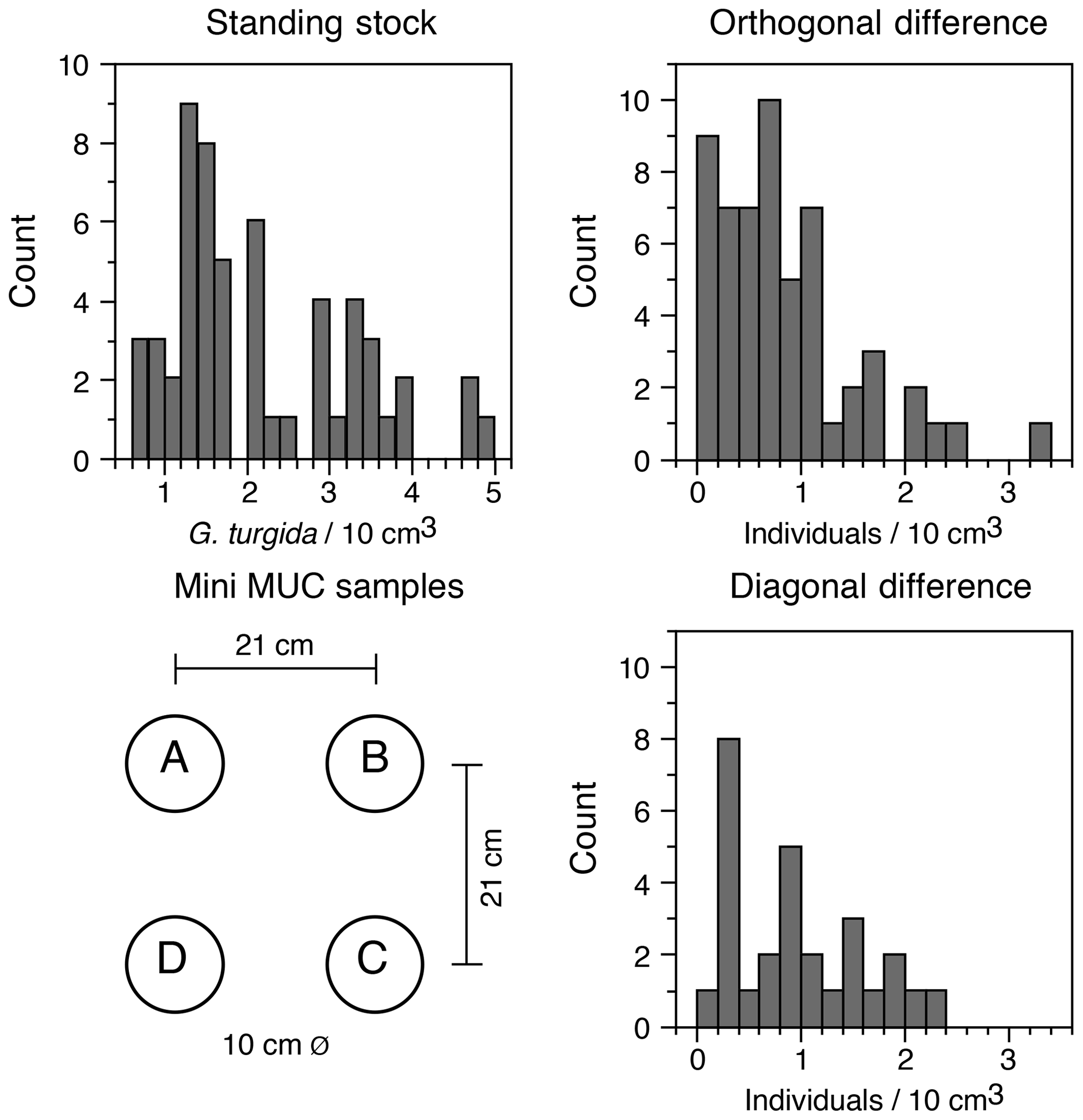
Figure 3 Frequency distribution of G. turgida standing stocks in the replicate samples and the differences between adjacent and diagonally located core samples. Replicate denominations and spatial dimensions of MiniMuc core samples are given for comparison.

Five of 15 deployments (OVS 290715-1, 290715-6; OVS 310715-1, 310715-5, and 310715-6) showed a substantially lower standing stock in one of the cores, whereas the G. turgida densities among the cores from the other 10 deployments were similar. The average difference of standing stocks between samples located diagonally in the core array of the MiniMuc was 1.0 specimens per 10 cm³ at 30 cm distance. The average density difference between adjacent cores was 0.8 specimens per 10 cm³ at 21 cm distance, which was slightly lower (Fig. 3). This difference could possibly mirror a patchiness at decimetre scales or more. The p value of a two-sample KS test was 0.55, indicating borderline significance for the orthogonal vs. diagonal differences in G. turgida standing stocks (Fig. 3). This suggests that the population densities were not substantially more different at a distance of 30 cm than at a distance of 21 cm.

The temporal data series showed G. turgida standing stocks ranging from 0.8 specimens per 10 cm³ in 2017 to 12.2 specimens per 10 cm³ in 2018. Earlier samples reported in the literature fell in this data range even though the size fractions >63 or 63–100 µm were analysed (Gustafsson and Nordberg, 2001; Risgaard-Petersen et al., 2006; Bergstrand, 2012). The mean value was 3.1±3.3 (1σ value, n=11) and hence substantially higher than in the replicate samples from 2015.

The p value of a KS test with Lilliefors modification was 0.077 for the temporal series standing stock data and 0.362 for the log-transformed data, both indicating a normal distribution. Once the very high standing stock of G. turgida in 2018 was omitted, the p values slightly increased to 0.098 or decreased to 0.286 for the log-transformed data. This again supported the hypothesis of a normal distribution, although with lower significance for the log-transformed data. This indicates that the temporal data were not adequately described by either normal or log-normal distributions. The log-probability plot indicates that G. turgida standing stocks from the temporal series are composed of two cohorts (a and b) with either comparatively high or low densities (Fig. 4c).

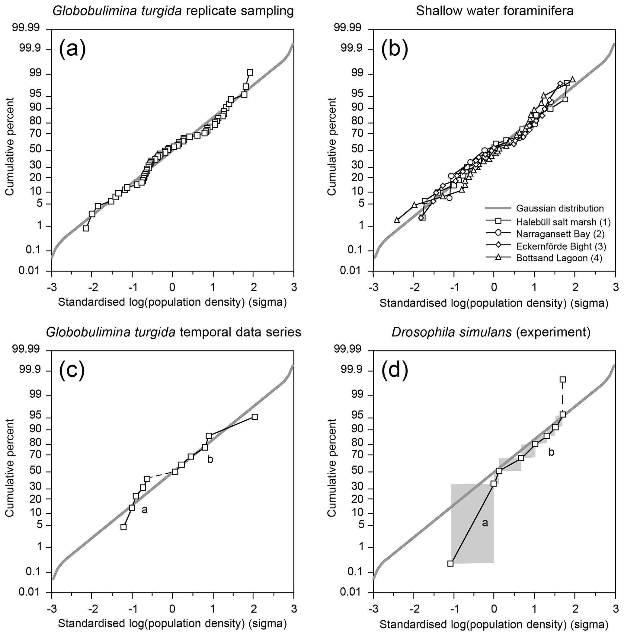
Figure 4 (a) Standardised population densities of (a) G. turgida, (b) shallow water foraminifers from replicate sampling, (c) the temporal series sampling, and (d) Drosophila simulans flies recorded in an ecological experiment on a log-probability scale and compared to a Gaussian distribution. The small characters “a” and “b” in panels (c) and (d) indicate different data subsets. Grey rectangles: range of binned data (Warren et al., 2006). Shallow water foraminiferal data sources: (1) Lehmann (2000, his Fig. 37), Ammonia beccarii ( A. tepida) >100 µm, Station P2, sampling on 11-8-1995, intertidal; (2) Brooks (1967, his Table 1), Ammonia beccarii >88 µm, Narragansett Bay, 20 m water depth; (3) Lutze (1968a, his Fig. 1), Elphidium excavatum >100 µm, Eckernförde Bight, 12 m water depth; (4) Lutze (1968a, his Fig. 6), Cribrononion articulatum (E.williamsoni) >100 µm, Bottsand lagoon, 0.2 m water depth.

3.3 Model simulation

The size, impedance, and spatial density of the potential patches were simulated with a model by Giddy Landan. None of the spatial structure models met the theoretical expectation of aggregations, and the hypothesis that they replicate the observed densities was rejected with high significance (Fig. 5). As an alternative to spatial structure, the fit of the empirical distribution pattern to several theoretical distributions was examined. In particular, we examined normal, log-normal, Gaussian mixture (with two to seven components), beta, gamma, logistic, log-logistic, exponential, and uniform distribution patterns. The best fit, as revealed by the Bayesian information criterion, was obtained with the log-normal distribution (Fig. 5). This was validated by the Lilliefors test that showed a p value of 0.22 and thus retained the null hypothesis that the logarithmically transformed data come from a normal distribution.

4 Discussion

4.1 Surface sediment heterogeneities at the Alsbäck Deep

The surface sediment in the deep Gullmar Fjord was a slightly clayey silt with a high proportion of medium-sized silt in the range of 8 to 22 µm. The sand-sized fraction >63 µm of near-surface sediments at Alsbäck Deep was less than 1 %, and the organic carbon content was 2.8 %–3 % (Hassellöv, 2001; Polovodova Asteman et al., 2013).

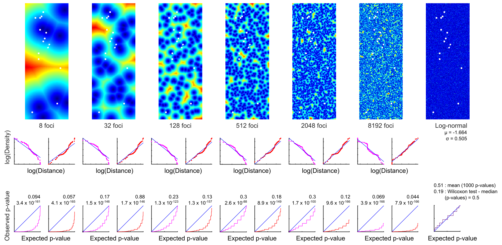
Figure 5 Modelling of G. turgida spatial structure. Top panels: example of six focal concentrations, i.e. putative patches (“pits” regime – dark blue: minimum, red: maximum population density), and a log-normal random sample without any spatial structure. Size of panels: 21×56 m, resolution 0.1 m. White quadruplets: MiniMuc deployments. Middle panels: relations of distribution functions between actual population densities and simulated distances from all 1000 replicates in one focal concentration. Magenta: the focal point is associated with maximal density (peaks). Red: the focal point is associated with minimal density (pits). Bottom panels: comparison of simulated and actual densities with the two-sided two-sample KS test. Blue lines: satisfactory model where the sorted p values produce a diagonal and the mean and median of Wilcoxon signed-rank test p values will be close to 0.5. The figure has been created by Giddy Landan.

Spatial heterogeneities of meiofauna abundances were reported to follow sedimentary inhomogeneities created by larger organisms or currents (e.g. Thrush, 1986; Buhl-Mortensen et al., 2010; Reiss et al., 2010; Hasemann and Soltwedel, 2011). The sediment surface at the Alsbäck Deep was often irregular and crumbly, and it showed burrows about a centimetre in diameter, which were also noticed in the near-surface sediment at a depth of 3 cm. Sediment in and around these burrows was often light brown to light olive-brown in colour as a result of bio-irrigation and oxygenation of otherwise oxygen-depleted sediments prevailing further down. Among macrofauna, centimetre-high polychaeta tubes were occasionally observed but other macro-organisms were rare (Appendix Table A1). Larger organisms creating structures at or beyond the scale of our MiniMuc cores were not recognised on the sediment surface retrieved by box cores during later sampling campaigns.

4.2 Ecology of Globobulimina turgida

Globobulimina species are commonly found living in intermediate to deep infaunal microhabitats (Corliss, 1985; Rathburn and Corliss, 1994; Bartels-Jonsdottir et al., 2006). They may also live on the sediment surface in areas where the flux rate of organic matter at the sea floor is high or the near-bottom water is low in oxygen (Lutze et al., 1986; Bernhard, 1992; Bernhard et al., 1997). Globobulimina species are common in oceanic or continental shelf environments, and they were also found in nordic fjords. Globobulimina auriculata including G. turgida morphotypes was rare in the Oslofjord, Norway (Hess et al., 2014), and it was occasionally common in the living fauna of the deep Hardangerfjord, Norway (Alve et al., 2011). A seasonal study performed at the Alsbäck Deep between 1993 and 1995 reported generally low abundances of living Globobulimina species. Higher numbers of G. auriculata were recorded in late March, early September, and December 1994, while G. turgida was generally found more often and showed higher abundances in early March, late July, and late September 1994, suggesting different reproduction windows for these two species (Gustafsson and Nordberg, 2001, their table 1).

Globobulimina species are well adapted to oxygen-depleted conditions (Bernhard and Alve, 1996), as there is evidence that they use nitrate instead of oxygen as a final electron acceptor for respiration (Risgaard-Petersen et al., 2006; Piña-Ochoa et al., 2010). Globobulimina turgida accumulates nitrate intracellularly. In order to restore the nitrate content in the cell, the specimens need to physically migrate through the sediment column to the zone where pore water nitrate is available rather than achieving this with the help of the pseudopodial network (Koho et al., 2011). The total intracellular nitrate accumulation in G. turgida is much higher under oxic conditions than during anoxia, which causes loss of intracellular nitrate for respiration through denitrification (Koho et al., 2011). Globobulimina species have been applied as palaeo-indicators for phases of oxygen depletion linked to weak intermediate or bottom-water ventilation or, together with other species, as indicators for periods of stronger surface ocean productivity (e.g. Lutze et al., 1986; Baas et al., 1998; Jorissen, 1999).

Even though Globobulimina species were related to a high flux of organic matter at the sea floor (e.g. Altenbach et al., 1999), they do appear to show a high degree of specialisation in exploiting different food resources. For instance, amorphous organic detritus was used by G. pacifica (Goldstein and Corliss, 1994), whilst bacteria that live around the redox boundary with a low concentration of phytodetritus were preferred by G. affinis (Schönfeld, 2001). The latter species sought and selectively ingested phytodetritus during a feeding experiment (Gooday, 2003; Nomaki et al., 2005). Also, nematodes were caught and found in the tests of G. auriculata, while fine-grained detritus was ingested by G. turgida s.s. centred inside a spherical cyst of its own reticulopodia (Cedhagen, 1996; Glock et al., 2019).

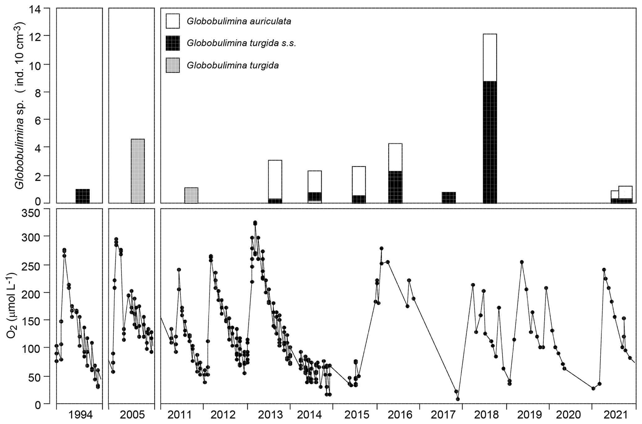
Figure 6 Temporal data series of Globobulimina sp. standing stock and near-bottom-water oxygen concentrations in the Alsbäck Deep in 1994, in 2005, and from 2011 through 2021. The data sources are provided in Supplement 2. Note that the columns in the upper panels are centred at the sampling dates.

The exploitation of different food sources and possibly different seasonal reproduction windows hypothetically sustained the coexistence of G. auriculata and G. turgida s.s. at the Alsbäck Deep for an extended period (Glock et al., 2019). The variations of their relative abundances could thus indicate changes in the ambient environmental conditions in the Gullmar Fjord, provided that the nematodes thrived under hypoxic conditions and were prey for G. auriculata. Indeed, nematodes react very sensitively to changes in oxygenation (Austen and Wibdom, 1991), and species adapted to hypoxia may increase in abundance under suboxic to anoxic conditions (e.g. Steyaert et al., 2007; Ingels et al., 2011). Nematode abundances also show patchiness on a centimetre scale, which is related to their locomotion and feeding behaviour rather than to aggregated heterogeneities of their food sources (Gallucci et al., 2009; Hasemann and Soltwedel, 2011).

The log-probability plot depicted temporal samples with high or low standing stocks of G. turgida as two different cohorts, hence indicating distinct ecological settings (Fig. 4c). Particularly, the standing stocks were comparatively high in 2005, 2013 through 2016, and 2018, whereas they were substantially lower in 2011, 2017, and 2021 (Fig. 6). During the period of higher absolute abundances, G. auriculata was more frequent than G. turgida s.s. from 2013 to 2015, whereas the latter was more frequent in 2018 (Appendix Table A3). The 2013 to 2015 samples were taken during an extended period of low-oxic to hypoxic bottom-water conditions in the Alsbäck Deep (Fig. 6). The 2018 sample was taken during a period of lower oxygen levels after a severe hypoxic event during winter 2017–2018 (Fig. 6; Choquel et al., 2021). Unfortunately, the regular monitoring programme of bottom-water oxygen concentrations in the Alsbäck Deep by the Swedish Meteorological and Hydrological Institute stopped in 2016. Only occasional data are available for the time since then (Fig. 6, Supplement 2). The dynamics of oxygenation in 2016 when both species were frequent and in 2017, when only G. turgida s.s. was present and very rare, are less constrained than in the years before. As such, a covariation of G. turgida standing stock or species abundance with bottom-water oxygenation cannot be established. On the other hand, the data suggest that Globobulimina species were more abundant when the previous low-oxygen period before the spring break-up ventilation phase was longer and more severe. This would indicate, however, that they grow rather slowly and may have reproduced about 1 year before the sampling.

Information on bacterial and nematode communities, as well as on phytodetritus concentrations in near-surface sediments at the Alsbäck Deep, was not available, excluding a comparison of G. turgida abundances with food availability (Altenbach et al., 1999). Therefore, it is not possible to gain further insight into the ecological conditions governing Globobulimina species living at the Alsbäck Deep. The timing of their reproduction and growth could be underlying factors structuring their abundance pattern.

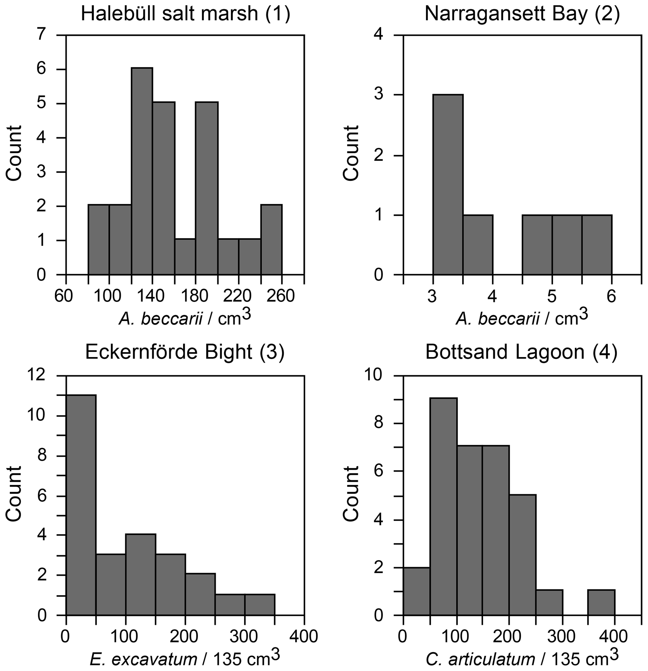
Figure 7 Frequency distribution of shallow water foraminiferal standing stocks in replicate sample series. Data sources are provided in Fig. 4.

4.3 Comparison with other foraminiferal data sets

A few foraminiferal data sets are available from the literature, suggesting an aggregated distribution of certain foraminiferal species. They comprise subtidal (Brooks, 1967; Lutze, 1968a) as well as intertidal environments (Buzas, 1968; Lehmann, 2000; de Chanvallon et al., 2015). The tightness of the patches appeared to be mirrored by bimodal frequency distribution histograms (Fig. 7). Samples outside of the patches were displayed as a maximum at population densities lower than the mean, whereas samples inside the patches showed a right-skewed maximum at values higher than the mean. Once the data were normalised to a logarithmic scale and compared with an ideal Gaussian distribution, they fit the latter with eye-catching accuracy (Fig. 4b). The log-normal fit was validated by non-significant p values in the Lilliefors test. This holds true for subtidal and intertidal species, and it remains consistent when a sampling location is revisited after 14 or 28 d. It also appears not to be related to the sample number. Therefore, log-normal distributions of foraminiferal species' population densities appear to be a pervasive feature of foraminifera, despite the substrate being mud, sand, or salt marsh soil and despite sampling in a contiguous (e.g. Lehmann, 2000), gridded (e.g. Lutze, 1968a), or random manner (e.g. Brooks, 1967).

4.4 Comparison with forced patchy distributions

Log-normal data distributions are characteristic of many volumetric variables (e.g. Schönfeld et al., 2021). They are recognised in foraminiferal populations, where high densities occur in a random pattern. This raises the question of which data distribution pattern prevails in an experimental setting under natural conditions where the spatial density of an organism is forced into a two-dimensional heterogeneity and high population densities are not randomly distributed. Surprisingly, such data are extremely sparse. Warren et al. (2003, 2006) reported an experiment on the occupation of nectarines by Drosophila simulans larvae. The fruit was arranged in a gridded array where half were shaded and half were exposed to direct sunlight. Both fruit setups were offered to small-sized insects. The substrate beneath the fruit including fly pupae was collected and the number of developed D. simulans was recorded. The spatial structure revealed a contagious distribution. The experiment revealed that significantly more flies per fruit developed on shaded nectarines than on those in the sun, probably due to a higher larval mortality at higher temperatures (Warren et al., 2006, their fig. 6). The standardised, binned fly abundances showed two subpopulations of data on a log-probability plot, which separate at a cumulative frequency of 50 % (Fig. 4d). The subpopulations are considered to depict two groups of flies, either developed under shaded or non-shaded nectarines. Their disjunct distribution of abundance data markedly differed from those of log-normal foraminiferal population densities from replicate sampling. Those indeed followed a Gaussian distribution on the log-probability plot and hence had to be considered a single cohort (Fig. 4a).

4.5 Constraints on the pulsating patch model

The concept of the pulsating patch model was based on early observations of asexual foraminiferal reproduction (e.g. Jepps, 1956). Juveniles often gathered around the dead parental test after schizogony, mainly to take up calcium and carbonate ions from the empty shell before they dispersed (Muller, 1974; Lutze and Wefer, 1980). The tightness of abundance maxima in contiguous sample series and the size distribution of the individuals suggested that the juveniles did not move very far from their point of origin (Buzas, 1968). Even consecutive reproduction events were preserved in one place. This enforced a pattern of ca. 1–2 cm sized patches with high population densities in salt marshes (Lehmann, 2000). However, several well-documented live observations of in-vitro asexual reproduction inferred that the juveniles disperse rapidly from the brood cyst at the parental test within minutes or hours (e.g. Murray, 2012). Soft-bottom-dwelling foraminifera may move several centimetres per day (e.g. Severin et al., 1982; Gross, 2000; Deldicq, 2021), which could lead to the establishment of another reproduction-induced abundance maximum at a different location. Consequently, a dynamic picture of pulsating patches in space and time emerges (Buzas et al., 2015).

The present study demonstrates that contiguous samples, to which the pulsating patchiness model has been applied (e.g. Buzas, 1968; Lehmann, 2000), showed a log-normal population density distribution. The distribution was the same as other data sets obtained from replicate sampling with greater distance between the replicates (Fig. 4). This result inferred important limitations of the pulsating patchiness model. First, the maxima mirrored discrete reproduction events that were randomly distributed on a wider scale. Second, these events occurred at a constant rate over time. These limitations are, however, rather an exception than the rule in nature: many benthic foraminifera show seasonal reproduction events that are linked to pulses of food supply or to the excess of certain temperature or salinity thresholds (Gooday, 1988; Lambshead and Gooday, 1990; Altenbach, 1992; Lutze and Wefer, 1980; Schönfeld and Numberger, 2007; Schönfeld, 2018). Food particles are not evenly distributed on the sea floor but scattered (e.g. Rice and Lambshead, 1994), which also promotes aggregated distributions of organisms using this food source. In essence, delineating patches at scales beyond the diameter of brood cysts or reproductive aggregations of juvenile specimens is, according to our results, truly artificial unless spatial statistics are applied in a sensible manner (de Chanvalon et al., 2022).

5 Conclusions

The present study differed in methodology and approach from previous investigations in the Gullmar Fjord. Living G. turgida were identified by their visual cytoplasm characteristics. Not less than 87 % of all living individuals were recognised in a particular sample when screening the residue submerged in seawater after washing. This recognition rate resembled the 90 % recovery rate reported from rose-bengal-stained faunas. The use of visual cytoplasm characteristics is therefore sufficiently reliable for the identification of G. turgida specimens that were living at the time of sampling. The examination of living specimens under water hampered the recognition of minute morphological differences between the closely related and genetically distinct species G. turgida s.s. and G. auriculata.

A total of 64 replicate 0–3 cm surface sediment samples were taken from a circle of 54 m diameter around the target location at the Alsbäck Deep, 60 of which could be quantitatively analysed and 58 yielded living G. turgida. The population densities depicted a log-normal distribution of G. turgida standing stocks. This was confirmed by a KS test with Lilliefors modification with high significance. The average difference of G. turgida standing stocks between samples located diagonally in the core array of the MiniMuc was higher than the average density difference between adjacent cores. A KS two-sample test showed borderline significance for orthogonal vs. diagonal standing stock differences, which challenged evidence for an aggregated distribution on a decimetre scale.

The sediment surface at the Alsbäck Deep was flat, and larger organisms creating structures at or beyond the MiniMuc core diameter were not recorded. Different patch sizes and patterns were created in an area of 21×56 m around the sampling sites with a numerical model. This model was then compared with the G. turgida standing stocks recorded. However, none of the known spatial structure models resembled the observed densities of our study species. The best fit was obtained with a random log-normal distribution. The hypothesis that G. turgida showed an aggregated distribution at larger scales was therefore rejected by statistical tests with high significance.

Patchy distribution patterns of benthic foraminiferal standing stocks from contiguous, gridded, or random sample replicates have been reported in the literature. A reanalysis of these data sets revealed log-normal distributions of foraminiferal standing stocks, which appeared to be a pervasive feature in all intertidal to nearshore environments. Delineating patches beyond the scale of reproductive agglomerations of juveniles around the parental test is therefore considered artificial. The use of spatial statistics may provide further insight once applicable to the data.

Standardised G. turgida standing stocks from the Alsbäck Deep replicate samples and literature data from other species and other locations depicted single cohorts on the log-probability plot. This matched a Gaussian distribution. Standing stocks of G. turgida from a temporal data series of living foraminiferal faunas from 1994 to 2021 showed two different cohorts on the log-probability plot. These data cohorts were related to samples with either high or low densities in different or consecutive years. Furthermore, data from a mesocosm experiment with D. simulans feeding on decaying nectarines where different microclimate treatments forced their abundance into a two-dimensional heterogeneity showed a similar data distribution pattern. The two data cohorts depicted by the log-probability plot are therefore considered to represent distinct ecological settings. The records of bottom-water oxygen concentrations in the Alsbäck Deep suggested a covariation of G. turgida standing stock or species abundances with bottom-water oxygenation during certain years. This relationship corroborates the conclusion that ecological or environmental forcing exerts a governing influence on the large-scale and temporal population structure of benthic foraminifera rather than their reproduction dynamics that act over a very fine scale.

Appendix A

Table A1 Coordinates, water depths, observations, and measurements at the replicate sampling stations at the Alsbäck Deep.

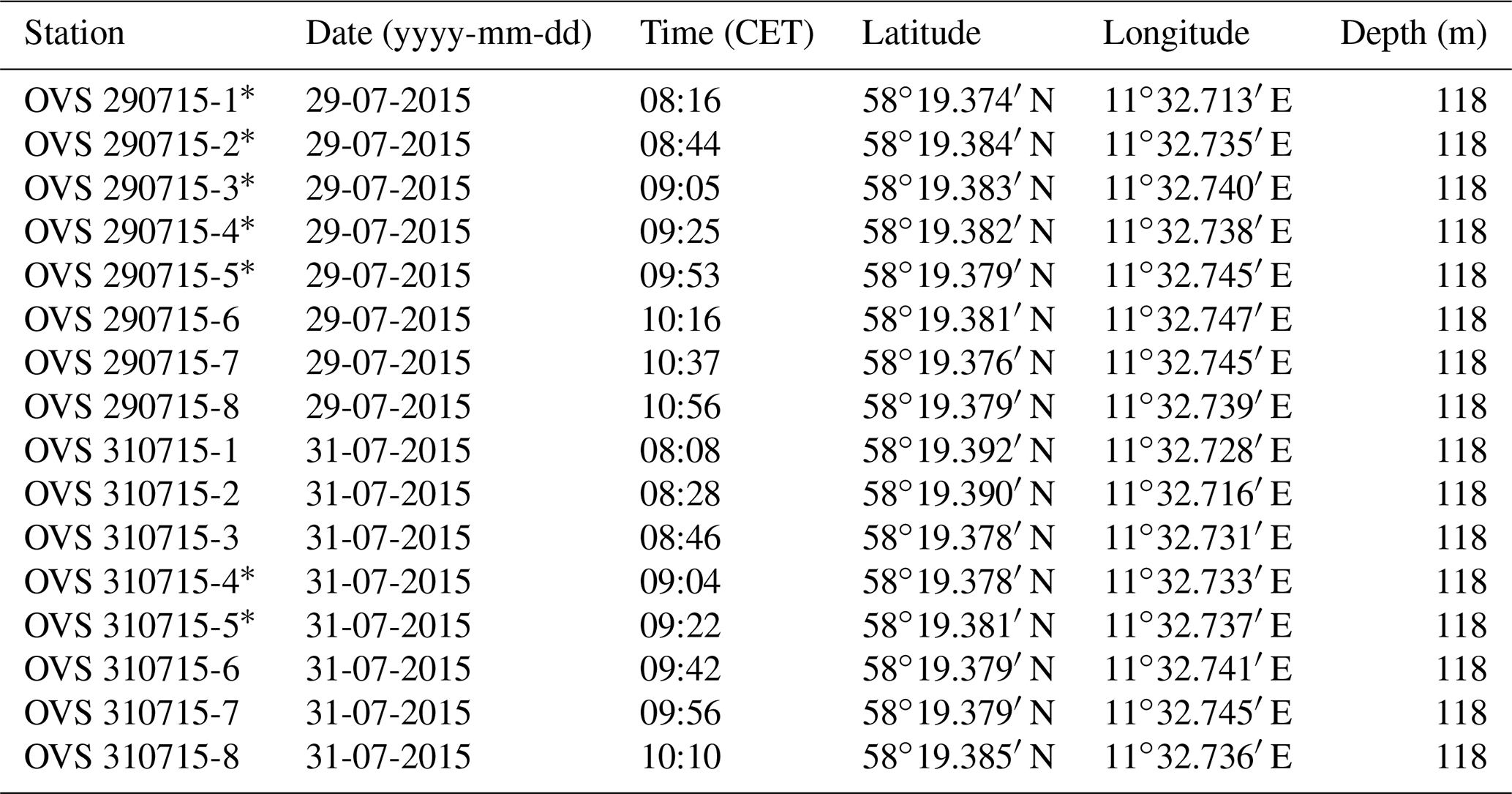
^∗ Observations and measurements – OVS 290715-1, core B: large tube worm; core C: surface sediment fluffy, disturbed. OVS 290715-2, core D: two worms. OVS 290715-3, core A: surface disturbed, sediment temperature 7.2 ^∘C; core D: worms, bottom-water salinity 34.1 units. OVS 290715-4, core D: bottom-water oxygen 66.7 µmol L⁻¹, value too high. OVS 290715-5, core A: worm; core B: clam. OVS 310715-4, core B: sediment temperature 7.1 ^∘C. OVS 310715-5, core D: bottom-water oxygen 50.7 µmol L⁻¹, value close to average, bottom-water salinity: 34.1 units.

Table A2 Census data, sample volumes, and standing stocks of G. turgida from the Alsbäck Deep sampling stations. SD: standard deviation. Numbers in brackets: the sample was not picked completely, and the number of specimens was not used in data analyses.

Table A3 Benthic foraminiferal census data from the temporal data series stations at the Alsbäck Deep.

(1) Gustafsson and Nordberg (2001): Alsbäck Deep, sampling date 28 July 1994, 116 m water depth, multicorer device with 75.4 cm² surface area, Station G116, composed of subsamples from 0–3 cm sediment depth, total sample volume 40.8 cm³, size fraction >63 µm, living fauna (rose bengal stained). (2) Bergstrand (2012): Gullmar Fjord, deep basin, sampling date 15 September 2011, 116 to 117 m water depth, Gemini corer with 50.3 cm² surface area, sample G113-11A, composed of subsamples from 0–3 cm sediment depth, size fraction 63–1000 µm, living fauna (rose bengal stained). (3) This study, sampling date 20 August 2013, 117 m water depth, composed of subsamples from 0–3 cm sediment depth, multicorer device, 78.5 cm² surface area, total sample volume 232 cm³, size fraction 125–2000 µm, $\mathrm{1}/\mathrm{4}$ split counted, living fauna (rose bengal stained). (4) This study, sampling date 30 July 2014, 117 m water depth, 0–3 cm sediment depth, MiniMuc device with 78.5 cm² surface area, size fraction 125–2000 µm, $\mathrm{1}/\mathrm{1}$ split counted, living fauna (rose bengal stained). (5) This study, sampling date 31 July 2015, 118 m water depth, 0–3 cm sediment depth, MiniMuc device with 78.5 cm² surface area, sample volume 295 cm³, size fraction 125–2000 µm, $\mathrm{1}/\mathrm{1}$ split counted, living fauna (rose bengal stained). (6) This study, sampling date 7 June 2016, 117 m water depth, 0–3 cm sediment depth, push core taken from a box corer, 43 cm² surface area, sample volume 120 cm³, size fraction 125–2000 µm, $\mathrm{1}/\mathrm{1}$ split counted, living fauna (rose bengal stained). (7) This study, sampling date 28 August 2017, composed of subsamples from 0–3 cm sediment depth, push core taken from a box corer, 41 cm² surface area, total sample volume 143 cm³, size fraction 125–2000 µm, $\mathrm{1}/\mathrm{1}$ split counted, living fauna (rose bengal stained). (8) This study, sampling date 15 August 2018, 117 m water depth, composed of subsamples from 0–3 cm sediment depth, push core taken from a box corer, 41 cm² surface area, total sample volume 80 cm³, size fraction 125–2000 µm, $\mathrm{1}/\mathrm{1}$ split counted, living fauna (rose bengal stained). (9) This study, sampling date 4 and 12 August 2021, 117 m water depth, composed of subsamples from 0–3 cm sediment depth, three push cores taken from a box corer, 41 cm² surface area, three separate gears, total sample volume 60 cm³, size fraction 125–5000 µm, $\mathrm{1}/\mathrm{1}$ split counted, living fauna (rose bengal stained). (10) This study, sampling date 29 September 2021, 117 m water depth, composed of subsamples from 0–3 cm sediment depth, three replicates taken by a Gemini corer, 50.24 cm² surface area, total sample volume 44, 45, and 34 cm³ (mean 41 cm³), size fraction 63–1000 µm, $\mathrm{1}/\mathrm{1}$, $\mathrm{1}/\mathrm{2}$ and $\mathrm{1}/\mathrm{1}$ split counted, living fauna (rose bengal stained). Data are mean values from replicate cores. Coordinates of replicate cores GC-A and GC-B are the same as given above, and coordinates of core GC-C are 58^∘19.399^′ N and 11^∘32.772^′ E.

Appendix B

The following are the taxonomic references of foraminiferal species from the Alsbäck Deep. Note: the genera and species are listed in alphabetical order. Their type references are given by Ellis and Messina (1940), the WoRMS Editorial Board (2023), and Loeblich and Tappan (1988). They are not included in the reference list of this paper.

•  

  Adercotryma glomerata (Brady, 1878) – Lituola glomerata Brady, p. 433, pl. 20, Fig. 1.

•  

  Ammodiscus gullmarensis Höglund, 1948, p. 45. Note: new name for Ammodiscus planus Höglund, 1947, p. 123, pl. 8, Figs. 2, 3, 8, pl. 28, Figs. 17, 18. The irregular coiling pattern of the last whorls discriminates Ammodiscus gullmarensis from other Ammodiscus species.

•  

  Ammonia beccarii (Linneì, 1758) – Nautilus beccarii Linneì, p. 710.

•  

  Ammonia tepida (Cushman, 1926) – Rotalia beccarii var. tepida Cushman, 1926, p. 79, pl. 1.

•  

  Bolivina dilatata Reuss, 1850, p. 381, pl. 48, Figs. 15a–c.

•  

  Bolivina gramen (d'Orbigny, 1839) – Vulvulina gramen d'Orbigny, p. 148, pl. 1, Figs. 30, 31.

  Bolivina pseudoplicata Heron-Allen and Earland, 1930, p. 81, pl. 3, Figs. 36–40.

•  

  Bolivina pseudopunctata Höglund, 1947, p. 273, pl. 24, Fig. 5, pl. 32, Figs. 23, 24.

•  

  Bolivina skagerrakensis Qvale and Nigam, 1985, p. 6–7, 10, pl. 1, Figs. 1–11, pl. 2, Figs. 1–10. Note: new name for Bolivina robusta Brady, 1881, p. 57, illustrated by Brady, 1884, p. 421, pl. 53, Figs. 7–9.

•  

  Bulimina marginata d'Orbigny, 1826, p. 269, pl. 12, Figs. 10–12.

•  

  Buliminella elegantissima (d'Orbigny) – Bulimina elegantissima d'Orbigny, 1839, p. 51, pl. 7, Figs. 13–14.

•  

  Cassidulina laevigata d'Orbigny, 1826, p. 282, pl. 15, Figs. 4, 5.

•  

  Cassidulina reniforme Nørvang, 1945 – Cassidulina crassa d'Orbigny var. reniforme Nørvang, p. 41, Figs. 6c–h. Note: the slightly inflated chambers and the characteristic beading on the outer margin of the final chamber, by which the aperture is located in a depression, discriminate this species from Cassidulina crassa.

•  

  Cibicides lobatulus (Walker and Jacob, 1798) – Nautilus lobatulus Walker and Jacob, p. 642, pl. 14, Fig. 36. Note: Lobatula lobatulus of authors.

•  

  Crithionina granum Goes, 1894, p. 15, pl. 3, Figs. 28–33. Note: Crithionina granum differs from C. pisum by the thin wall and elongated shape of the tests.

•  

  Cribrononion articulatum (d'Orbigny, 1839) – Polystomella articulata d'Orbigny, p. 30, pI. 3, Figs. 9,10.

•  

  Eggerelloides advena (Cushman, 1922) – Verneuilina advena Cushman, p. 9, pl. 1, Fig. 5.

•  

  Eggerelloides medius (Höglund, 1947) – Verneuilina media Höglund, p. 184, pl. 13, Figs. 7–10, pl. 30, Fig. 21. Note: the coarse agglutination, less distinct chamber walls, and stout shape allow the differentiation of this morphospecies from Eggerelloides scaber in the Gullmar Fjord assemblages.

•  

  Eggerelloides scaber (Williamson, 1858) – Bulimina scabra Williamson, p. 65, pl. 5, Figs. 136, 137.

•  

  Elphidium albiumbilicatum (Weiss) – Nonion pauciloculum Cushman subsp. albiumbilicatum Weiss, 1954, p. 157, pl. 32, Figs. 1, 2.

•  

  Elphidium clavatum Cushman, 1930, p. 20, pl. 7, Fig. 10. Note: Elphidium excavatum of Bergstrand (2012). The specimens from the Alsbäck Deep show a distinct knob or a few larger granules in the umbilicus and more chamber projections bridging the sutures compared to Elphidium excavatum individuals from the Gullmar Fjord are less stout compared to specimens from the Baltic Sea (Lutze, 1965; Polovodova et al., 2009). The species identification is corroborated by Darling et al. (2016), who recorded the Elphidium genotype S4 (= E. clavatum) at the Alsbäck Deep.

•  

  Elphidium incertum (Williamson, 1858) – Polystomella umbilicatula var. incerta Williamson, p. 44, pl. 3, Figs. 82, 82a. Note: the specimen shows a fine granulation in the umbilical area and inner part of the sutures. The sutures are not that oblique and the umbilical area is smaller than in Elphidium magellanicum.

•  

  Elphidium magellanicum (Heron-Allen and Earland, 1932) – Elphidium (Polystomella) magellanicum Heron-Allen and Earland, p. 440, pl. 16, Figs. 26–28.

•  

  Elphidium williamsoni Haynes, 1973, p. 207, pl. 27, Fig. 7, pl. 25, Figs. 6, 9, pl. 27, Figs. 1–3. Note: Cribrononion articulatum or Cribrononion cf. alvarezianum of authors (Lutze, 1968b).

•  

  Epistominella vitrea Parker, 1953, p. 9, pl. 4, Figs. 34–36.

•  

  Evolvocassidulina bradyi (Norman, 1881) – Cassidulina bradyi (Norman), Brady, p. 59, illustrated by Brady (1884), pl. 54, Figs. 6–10.

•  

  Globobulimina auriculata (Bailey, 1851) – Bulimina auriculata Bailey, p. 12, Figs. 25–27.

•  

  Globobulimina turgida (Bailey, 1851) – Bulimina turgida Bailey, p. 12, Figs. 28–30, 67.

•  

  Haplophragmoides bradyi (Robertson, 1891) – Trochammina bradyi Robertson, p. 388. Note: new name for Trochammina robertsoni Brady 1887, p. 893, pl. 20, Fig. 4.

•  

  Haynesina germanica (Ehrenberg) – Nonionina germanica Ehrenberg, 1840: p. 23, pl. 2, Fig. 1a–g.

•  

  Hyalinea balthica (Schröter, 1783) – Nautilus balthicus Schröter, p. 20, pl. 1, Fig. 2.

•  

  Islandiella norcrossi (Cushman, 1933) – Cassidulina norcrossi Cushman, p. 7, pl. 2, Fig. 7.

•  

  Lagena laevis (Montagu, 1803) – Vermiculum laeve Montagu, p. 524., pl. 1, Fig. 9.

•  

  Liebusella goesi Höglund, 1947, p. 194, pl. 14, Figs. 4–8.

•  

  Lagena clavata (d'Orbigny, 1846) – Oolina clavata d'Orbigny, p. 24, pl. 1, Figs. 2–3.

•  

  Lenticulina atlantica (Barker) – Robulus atlanticus Barker, 1960, p. 144, pl. 69, Figs. 10–12. Note: new name for Cristellaria lucida Thalmannn, 1937.

•  

  Leptohalysis scotti (Chaster 1892) – Reophax scottii Chaster, p. 57, pl. 1, Fig. 1.

•  

  Miliolinella subrotunda (Montagu, 1803) – Vermiculum subrotundum Montagu, p. 521.

•  

  Nonionella stella Cushman and Moyer, 1930 – Nonionella miocenica Cushman var. stella Cushman and Moyer, p. 56, pl. 7, Fig. 17a–c. Note: the name Nonionella sp. T1 has been proposed for N. stella morphospecies from the Gullmar Fjord (Deldicq et al., 2019) because the SSU rDNA sequences from specimens collected in the Gullmar Fjord, Oslofjord, and Skagerrak differ from a gene sequence obtained from an N. stella specimen from the Santa Barbara Basin, California Borderland, at 594 m water depth (Bernhard et al., 2006). Unless gene sequences from topotypic specimens are available, i.e. the continental shelf off San Pedro, California, at 64 to 92 m water depth, we keep with the denomination as Nonionella stella.

•  

  Nonionella turgida (Williamson, 1858) – Rotalina turgida Williamson, p. 50, pl. 9, Figs. 95–97.

•  

  Nonionellina labradorica (Dawson 1860) – Nonionica scapha var labradorica Dawson, p. 191, pl. 4.

•  

  Pateoris hauerinoides (Rhumbler, 1936) – Quinqueloculina subrotunda forma hauerinoides Rhumbler, pp. 206, 217, 226.

•  

  Nummuloculina irregularis (d'Orbigny) – Biloculina irregularis d'Orbigny, 1839, p. 67, pl. 8, Figs. 20, 21.

•  

  Polystomammina nitida (Brady, 1881) – Trochammina nitida Brady, p. 52, pl. 41, Figs. 5a–c, 6.

•  

  Psammosphaera bowmanni Heron-Allen and Earland, 1912, p. 385, pl. 5, Figs. 5, 6.

•  

  Pyrgo williamsoni (Silvestri, 1923) – Biloculina williamsoni Silvestri, p. 73, pl. 6, Figs. 169, 170.

•  

  Pyrgoella sphaera (d'Orbigny, 1839) – Biloculina sphaera d'Orbigny, p. 66, pl. 8, Figs. 13–16.

•  

  Quinqueloculina seminulum (Linné, 1758) – Serpula seminulum Linné, p. 786.

•  

  Quinqueloculina stalkeri Loeblich and Tappan, 1953, p. 40, pl. 5, Figs. 5–7, 9.

•  

  Recurvoides trochamminiforme Höglund, 1947, p. 149, pl. 11, Figs. 7–8, pl. 30, Fig. 23.

•  

  Reophax dentaliniformis Brady, 1881, p. 49, illustrated by Brady, 1884, pl. 30, Figs. 21, 22.

•  

  Reophax fusiformis (Williamson, 1858) – Proteonina fusiformis Williamson, p. 1, pl. 1, Fig. 1.

•  

  Reophax subfusiformis Earland, 1933, p. 74, pl. 2, Figs. 16–19. Note: this species differs by the exponential increase in chamber size, moderately oblique sutures, and narrowly curved initial part of the test from Reophax fusiformis, which shows strongly oblique sutures, a moderate increase in chamber size, and a gently curved test shape.

•  

  Rosalina anomala Terquem, 1875, p. 20, pl. 5, Figs. 1a–b.

•  

  Stainforthia fusiformis (Williamson, 1858) – Bulimina pupoides d'Orbigny var. fusiformis Williamson, p. 63, pl. 5, Figs. 129, 130.

•  

  Spiroplectammina biformis (Parker and Jones, 1865) – Textularia agglutinans var. biformis Parker and Jones, p. 370, pI. 15, Figs. 23, 24.

•  

  Stainforthia concava (Höglund, 1947) – Virgulina concava Höglund, p. 257, pl. 23, Figs. 3a, b, 4a, b, pl. 32, Figs. 4–7, text Figs. 273–275.

•  

  Textularia pseudogramen Chapman and Parr, 1937, p. 153.

•  

  Textularia earlandi Parker, 1952, p. 458. Note: new name for Textularia tenuissima Earland, 1933, p. 95, pl. 3, Figs. 21–40.