Radiolarian assemblages related to the ocean–ice interaction around the East Antarctic coast

The Southern Ocean plays a central role in Earth's climate, ecology, and biogeochemical cycles. Therefore, understanding long-term changes in Southern Ocean water masses in the geologic past is essential for assessing the role of the Southern Ocean in the climate system. Radiolarian fossils are a useful tool to reconstruct the water masses of the Southern Ocean. However, the radiolarian assemblages in the high latitudes of the Southern Ocean (south of the polar front (PF)) are still poorly understood. In this paper, we report the radiolarian assemblages in surface marine sediment and plankton tow samples collected from the high latitudes south of the PF.

In the surface sediments, four factors (named F1–F4) of the radiolarian assemblages were identified using Q-mode factor analysis, which are related to different water masses and hydrological conditions. F1 is related to the surface waters south of the southern boundary (SB) of the Antarctic Circumpolar Current (ACC), which are cooled by melting sea ice and ice sheets. F2 is associated with water masses north of the SB. A comparison with the vertical distribution of the radiolarian assemblages in plankton tow samples indicates that characteristic species are associated with the Circumpolar Deep Water (CDW) and surface waters north of the SB. F3 is associated with modified Circumpolar Deep Water (mCDW). The radiolarian assemblage of F4 does not seem specifically related to any of the water mass here analyzed. However, the species in this assemblage are typically dwells within ice shelf and/or sea ice edge environments. Radiolarian assemblages here identified and associated with water masses, and ice edge environments are useful to reconstruct the environment south of the PF in the geologic past.

1 Introduction

The interaction between the Southern Ocean and the Antarctic Ice Sheet plays an important role in the global climate system. Recently, it has been revealed that an increase in warm seawater intrusion under the ice shelf results in substantial melting of the Antarctic Ice Sheet (Rignot et al., 2013), potentially leading to a significant rise in global sea levels in the future (DeConto and Pollard, 2016). Melting of the ice sheet and sea ice also triggers a reduction in the formation of Antarctic Bottom Water (AABW), which is an important component of the global climate system (e.g., Hayes et al., 2014). Gaining insight into the hydrographic dynamics resulting from the interaction between the Southern Ocean and the Antarctic Ice Sheet is crucial for a better understanding of the global climate system. Furthermore, investigating the temporal change in the Antarctic Ice Sheet responses to the oceanic forcing is necessary to understand the long-term interactions between the Southern Ocean and the Antarctic Ice Sheet.

Foraminifera fossils in marine sediments have been used to reconstruct the past change in the volume of water masses distributed in the Southern Ocean (e.g., Hayes et al., 2014). While calcareous microfossils like foraminifers and their geochemical analyses are valuable tools for paleoceanographic studies, their use in the Southern Ocean is limited because of the widespread presence of carbonate-free sediments south of the polar front (PF). It is well known that siliceous microfossils, such as radiolarians and diatoms, are common in the sediments south of the PF (Dutkiewicz et al., 2015). Polycystine radiolarians (hereafter radiolarians) are one group of planktonic microorganisms (Protista) that are distributed in the world's oceans, and their siliceous skeletons are preserved in deep-sea sediments as microfossils. Because radiolarian assemblages and their geographical and vertical distributions are closely related to the oceanic environments, they have been widely used as a paleoceanographic proxy (e.g., Cortese and Abelmann, 2002; Abelmann and Gowing, 1997; Matsuzaki et al., 2016).

To apply this method in high latitudes, it is essential to have information on the relationship between radiolarian assemblages and hydrography in this region. However, most previous studies focusing on radiolarian assemblages have been conducted north of the southern boundary (SB) of the Antarctic Circumpolar Current (ACC), and information on radiolarian assemblages south of the SB is limited (Lawler et al., 2021; Abelmann et al., 1999; Abelmann and Gowing; 1997; Morley and Stepien, 1985). While radiolarian assemblages in sediments have been already reported in the East Antarctic sector (Nishimura et al., 1997; Nishimura and Nakaseko, 2011), they have not yet been related to the water masses properties.

This study aims to (1) provide information on the radiolarian assemblages from the continental shelf to the abyssal plain south of the PF and (2) clarify their relation to water masses. This study especially focuses on the water mass around the East Antarctic coastal areas, where radiolarian data are scarce.

2 Regional setting

2.1 Geographic setting

The study area covers the continental shelf to the abyssal plain in East Antarctica south of the PF (water depth ranging from 219 to 4642 m) (Fig. 1; Table 1). Regarding the surface sediment sampling in this study, the study area is divided into three subareas, i.e., the Cosmonauts Sea, the Cooperation Sea, and the Mawson Sea (Fig. 1b).

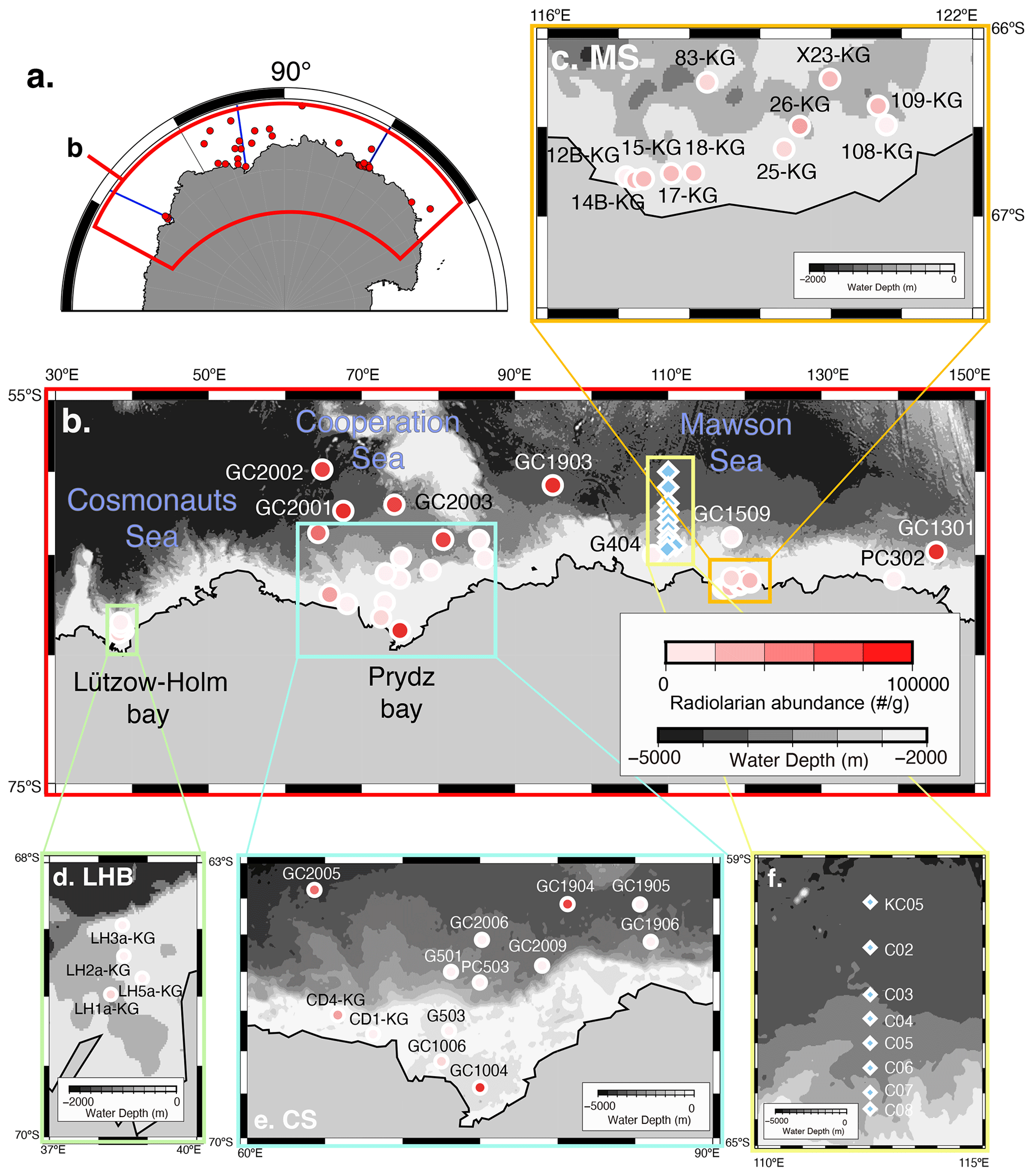
Figure 1 Map of the Southern Ocean showing the sample location. (a) Map of Antarctica. Red dots are sample locations used in this study. The blue line is the vertical section in Fig. 2. (b) Distribution of radiolarian abundance in surface sediment samples. Light blue diamonds are plankton tow sample locations. (c, d, e) Close-up of the map in Fig. 1b in the Sabrina Coast (SC), Lützow–Holm Bay (LHB), and Cooperation Sea (CS), respectively. (f) Close-up of the map in the plankton tow sample location. Five maps (b, c, d, e, f) showing previously published data overlain on the Bedmap2 subglacial topography (Fretwell et al., 2013).

Table 1 Locations and water depth of samples.

The Cosmonauts Sea, situated between 30 and 50^∘ E in the Southern Ocean (Fig. 1b), encompasses Lützow–Holm Bay (LHB). This bay is characterized by a deep glacial trough in the center that is ∼ 15 km wide and more than 600 m deep and deepens southward to ∼ 1200–1400 m (Hirano et al., 2020). To the east of the Cosmonauts Sea lies the Cooperation Sea, which includes Prydz Bay (PB). Prydz Bay is a vast embayment covering an area of approximately 80 000 km². Within Prydz Bay, the continental shelf slopes gradually toward the land, with water depths ranging from approximately 200 to 400 m at the continental shelf break, increasing to about 600 to 1000 m at the inner shelf (Fretwell et al., 2013). The Mawson Sea, situated to the east of the Cooperation Sea, encompasses the Sabrina Coast (SC). The continental shelf in the Sabrina Coast region is typically over 120 km wide (Close et al., 2007). The topography in the SC is similar to that of PB and LHB, with the seabed deepening landwards from the outer shelf at depths ranging from 200 to 500 m to inner shelf depths exceeding 1400 m in this study area of SC (116–122^∘ E).

2.2 Oceanographic setting

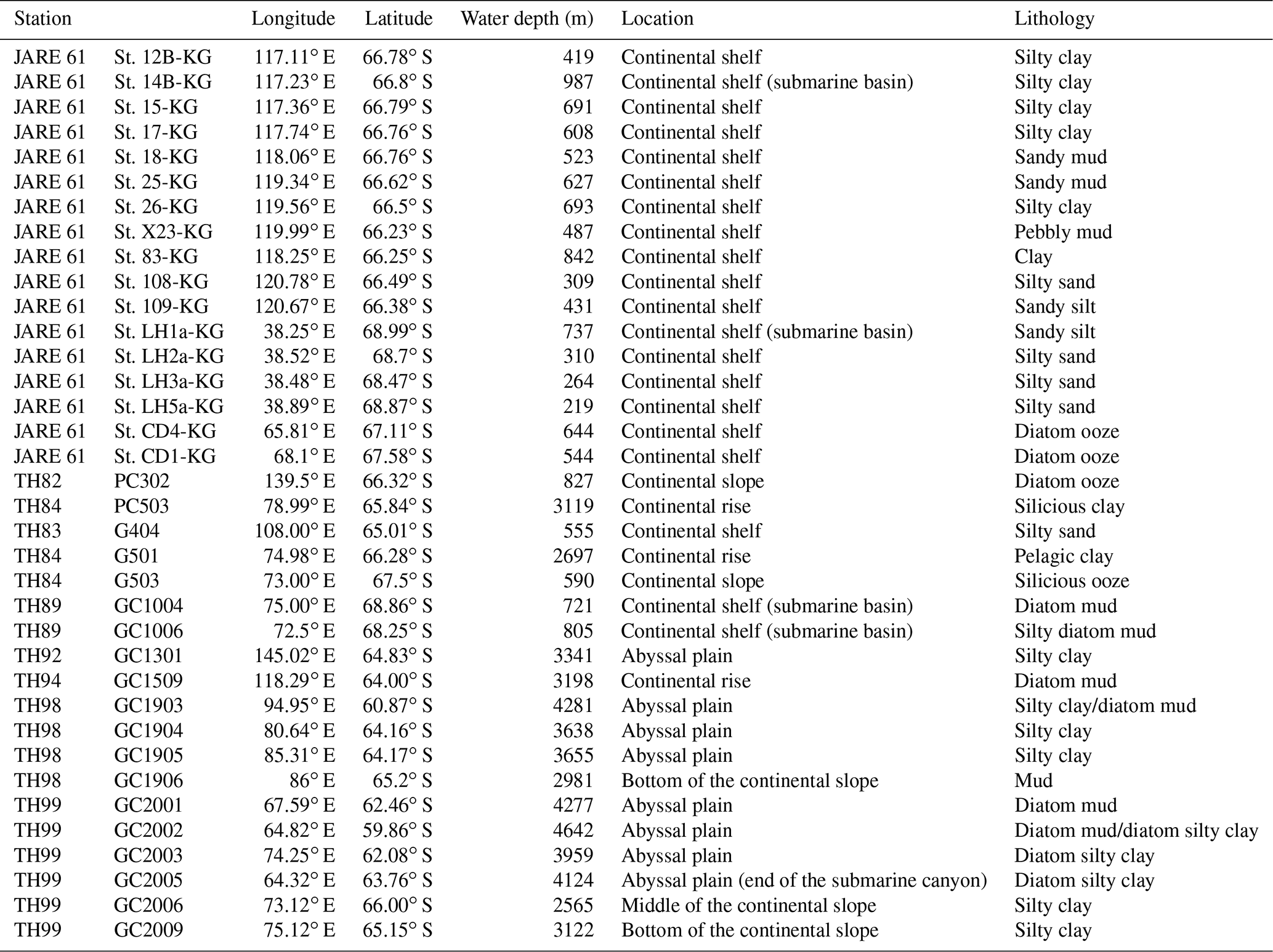
The Southern Ocean south of the PF is mainly occupied by three water masses, i.e., Antarctic Surface Water (AASW), Circumpolar Deep Water (CDW), and AABW (Fig. 2). The AASW is a cold and low-salinity mass that forms at the surface south of the PF (Fig. 2). To the north of the southern boundary (SB), the surface water temperature rises to approximately 0 ^∘C due to summer solar radiation, and the subsurface cold layer (often referred to as winter water) is relatively thin and not extremely cold. South of the SB, the subsurface cold layer, which formed in winter at nearly −2 ^∘C is much thicker (Fig. 2). CDW is a warm (1.5–3 ^∘C) and salty (salinity ∼ 34.7) water mass located below a water depth of 2000 m north of 40^∘ S and is mainly derived from North Atlantic Deep Water. South of 40^∘ S, CDW shoals due to wind-driven upwelling (Greene et al., 2017; Marshall and Speer, 2012). As CDW moves poleward, it undergoes mixing with AASW and continental shelf waters, leading to a modification of its core properties (Orsi and Wiederwohl, 2009), resulting in what is known as modified Circumpolar Deep Water (mCDW). AABW is a water mass generally occurring below 4000 m, with temperatures ranging from −0.8 to 0 ^∘C and salinities ranging from 34.6 to 34.7. AABW, which originates from mCDW and dense shelf water characterized by temperatures as low as −1.8 ^∘C and high salinity (>34.6), is formed in various Antarctic coastal polynyas, including those in the Adélie Coast (Mertz Polynya) and Prydz Bay (Cape Darnley polynya).

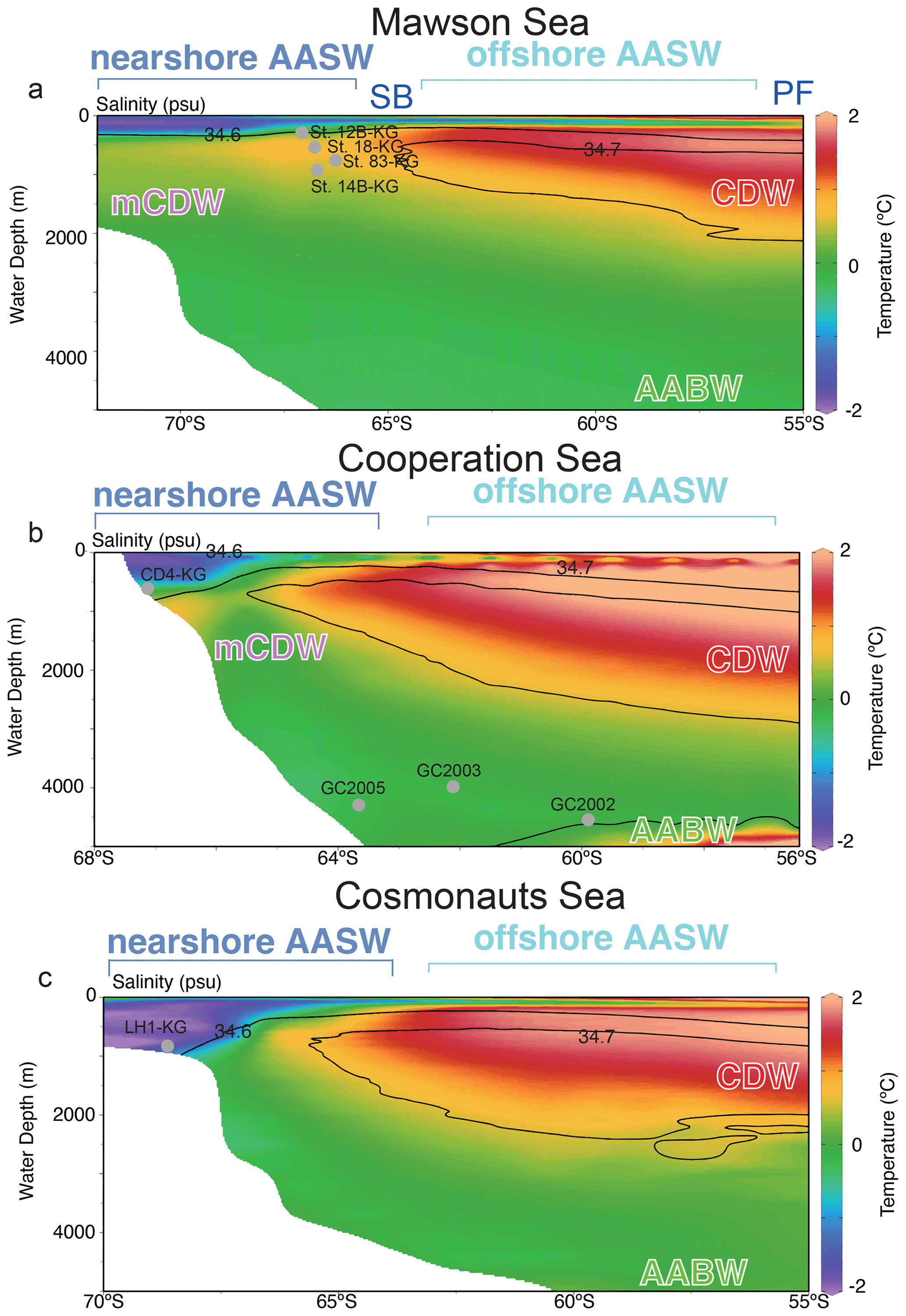
Figure 2 Vertical section along the blue line in Fig. 1. Color-mapped temperature, with salinity contours overlain, as drawn from the 2018 World Ocean Atlas. In this study area, the major fronts are the polar front (PF), and southern boundary of Antarctic Circumpolar Current (SB), and major water masses are Antarctic Surface Water (AASW), Circumpolar Deep Water (CDW), and modified CDW (mCDW). Gray points are representative site locations (depth and latitude). Figures are made using the software Ocean Data View (ODV) 5.6.7 of Schlitzer (2021). Temperature and salinity data are from the World Ocean Atlas 2018 of Locarnini et al. (2018) and Zweng et al. (2019).

The water structure on the continental shelf region is affected by different processes, such as mCDW intrusion, sea ice formation in polynyas, and freshwater discharge from ice shelves. In this study area, polynyas (Dalton and Cape Darnley polynyas; Fig. 1) are present in SC and PB (Tamura et al., 2008). In LHB, mCDW (>0 ^∘C) intrudes the continental shelf along the trough (Hirano et al., 2020). In SC, mCDW also intrudes the continental shelf along the depression from east to west, with the near-surface cold layer largely affected by Dalton Polynya (Silvano et al., 2018). Conversely, the intrusion of mCDW is less pronounced in the Prydz Bay (PB) area, primarily due to significant winter heat loss in this region (Herraiz-Borreguero et al., 2015; Guo et al., 2019).

3 Materials and methods

3.1 Surface sediment

A total of 36 surface sediment samples (0–2 cm depth) from the area of 59–68^∘ S and 38–145^∘ E (water depths ranging from 219 to 4642 m) were used in this study (Fig. 1; Table 1). There were 17 samples collected from the continental shelf, using a grab sampler during the 61st Japanese Antarctic Research Expedition (JARE-61) cruise of icebreaker (I/B) Shirase in 2019–2020. Then, 19 samples were collected from the continental shelf, continental slope, and abyssal plain during cruises conducted by the Japan National Oil Corporation as part of the Antarctic Geological and Geophysical Research Project (1989–2000) aboard R/V Hakurei Maru, using piston or gravity corers. Their core top samples were used as surface sediments.

Freeze-dried subsamples were weighed (approximately 1–2 g), treated with 15 % H₂O₂ to remove the organic matter, and then treated with an HCl solution to remove the calcium carbonate. The samples were then wet-sieved (45 µm mesh size), after which two types of permanent slides were made from the residue to quantify the abundance (Q-slide) and for faunal analysis (F-slide) using the method described by Itaki et al. (2018). Briefly, the Q-slides were prepared by transferring all residue to a 200 mL beaker containing 100 mL distilled water. The solution was well mixed, and a 0.5 mL sample was taken from the suspension using a micropipette and dropped onto a glass slide. The sample was then dried and mounted with Norland Optical Adhesive. The F-slides were made from the remaining residues in the beaker and then mounted.

Radiolarian skeletons were observed under an optical microscope at 100×, 200×, and 400× magnifications. The radiolarian concentration, which represents the total number of radiolarians present in 1–2 g of dry sediment, was estimated using the following equation: RC (specimens g⁻¹) is equal to the total number of specimens in the Q-slide × 200 $/$ sample weight (g). The relative abundance (percent of total assemblage) of radiolarian taxa was estimated by counting and identifying more than 300 specimens on the F-slide; however, as many individuals as could have been identified were counted in the F-slide when radiolarian abundances were scarce.

3.2 Plankton tow samples

A plankton tow with a mesh size of 60 µm and a collecting and closing system (with a frame diameter of 1 m) was vertically towed at eight stations in the Mawson Sea of the Southern Ocean (Fig. 1) during the 16th Kaiyodai Antarctic Research Expedition aboard training vessel (TV) Umitaka Maru in January 2013. At all stations, three–four vertical tows were carried out at a maximum speed of 0.5 m s⁻¹ through intervals of 0–50, 50–100, 100–200, and 200–500 m. A calibrated flow meter (Rigosya, Japan) was employed to determine the volume of filtered water.

The plankton samples were preserved in borate-buffered formalin–seawater solution (final concentration 5 %) and were stained with rose bengal to distinguish living specimens from dead ones. Observation slides were prepared using the following process. First, larger zooplankton were excluded from the original samples using a 1 mm mesh. Second, specimens smaller than 1 mm were split into aliquots between $\mathrm{1}/\mathrm{16}$th and $\mathrm{1}/\mathrm{128}$th of the original quantity. Third, specimens were wet-sieved using a 45 µm mesh. Finally, the sample was dried and mounted with Norland Optical Adhesive. Polycystine radiolarian species were identified and counted using an optical microscope at magnifications of 100× or 200×. All plankton specimens on a slide were identified and counted, and their individual counts were converted to abundance (number of specimens per m³).

3.3 Temperature and salinity profiles

During the JARE-61 cruise, vertical hydrographic data, including temperature, salinity, and dissolved oxygen (DO), were collected using a conductivity–temperature–depth profiler (CTD) (Sea & Sun Technology CTD90M), which was equipped with the grab sampler. Salinity and DO values were calibrated using regression lines derived from salinity and DO data obtained from both Niskin bottle bottom-water samples and a sensor installed in the grab sampler.

The hydrographic dataset (including temperature, salinity, and DO) from the World Ocean Atlas 2018 was also utilized to depict the distribution of water masses across a broad region. Although these hydrographic datasets provided annual, winter, spring, summer, and autumn data, the austral summer datasets were used to compare with the austral summer data observed by the JARE-61 cruise. In addition, the austral summer datasets were used because sediment trap studies in the Southern Ocean have demonstrated that radiolarian flux in austral summer contributes most of the annual flux (Abelmann and Gersonde, 1991; Abelmann, 1992).

3.4 Q-mode factor analysis for surface sediments

A Q-mode factor analysis (Imbrie, 1971; Imbrie et al., 1973) was conducted on surface sediment samples to illustrate the relationships between oceanographic conditions in each factor analysis interval and the ecology of the radiolarians found in those intervals. For factor analysis, the size of the dataset of counted radiolarians was reduced to a total of 24 taxa. In accordance with the procedure outlined by Abelmann and Gowing (1997), species with abundances below 1 % and those occurring in only one or two samples with abundances below 2 % were removed from the dataset. The groups of juvenile nassellarians and spumellarians, which could not be identified at the species level, were not included in the statistical data. Moreover, the dataset was simplified by consolidating certain taxa to minimize counting uncertainties and enhance the reproducibility of counts for taxa with intricate taxonomy (e.g., Acanthosphaera spp.). Among the 36 samples, 17 had fewer than 100 radiolarians on the F-slide and were excluded from subsequent analyses. In the remaining 19 samples, between 100 and 300 specimens were identified at the species level. The PAST statistical software package (Paleontological Statistics v. 4.4) (Hammer et al., 2001) was used for the Q-mode factor analysis. Prior to the analysis, the data were normalized, following the method described by Itaki et al. (2008, 2010).

4 Results

4.1 Hydrography

AASW with low temperature (−2 to 1 ^∘C) and low salinity (∼ 34.5) was observed in the surface layer (∼ 400 m) at all continental shelf sites south of SB (Fig. 3) (hereafter nearshore AASW). In certain locations on the continental shelf of PB and SC, relatively warmer water (around 1 ^∘C) was present in the surface layer (upper 100 m) as a result of summer solar heating. This warm surface water was particularly prominent in the polynya areas, such as St. X23-KG and St. CD4-KG (refer to the Supplement). In addition, the surface layer (upper 100 m) had low salinity (33.2–34.2) due to meltwater from sea ice and glacial ice at most sites. In the abyssal plain area north of SB, the temperature in AASW, which occupies the surface layer (upper 100 m), increased from south to north (Fig. 2) (hereinafter offshore AASW).

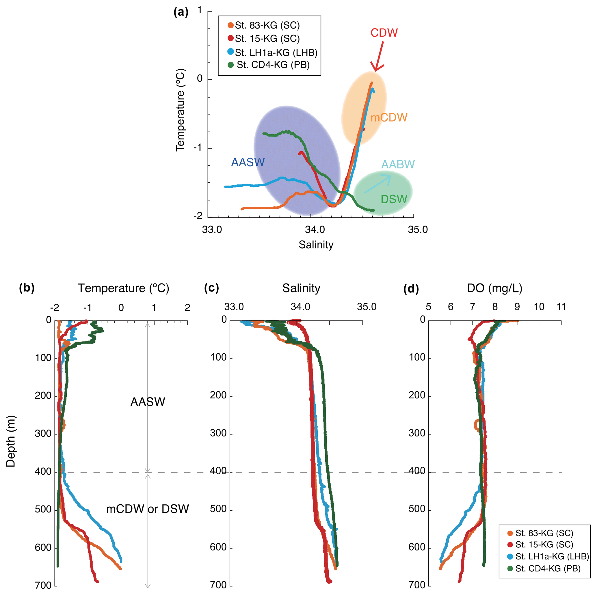
Figure 3 Temperature and salinity profiles. (a) Example of temperature and salinity profiles in each area (smoothed data), including the information of the water masses. (b) Example vertical profiles of temperature, salinity, and dissolved oxygen in each area. AASW is the Antarctic Surface Water; CDW is the Circumpolar Deep Water; mCDW is the modified Circumpolar Deep Water; AABW is the Antarctic Bottom Water; DSW is the dense shelf water.

CDW with high salinity (∼ 34.7) and warm temperature (1–2 ^∘C) was observed below AASW in the abyssal plain sites north of SB (water depth of 200–3000 m). This CDW shoaled toward the south due to wind-driven upwelling (Fig. 2). Warm and high salinity water below 400 m was observed at continental shelf sites in SC and LHB, reflecting mCDW intrusion into the continental shelf. In particular, high temperature (>0 ^∘C) was observed at St. 83-KG and St. X23-KG (Fig. 3; see the Supplement), indicating a significant intrusion of relatively warm mCDW into these sites. At St. LH1a-KG, relatively warm (>0 ^∘C) water was recognized in the bottom layer, indicating an intrusion of mCDW (Fig. 3; see the Supplement).

Conversely, in the PB area, the bottom layer is marked by high salinity (>34.5) and low temperature (< −1.5 ^∘C) (Fig. 3), signifying the presence of dense shelf water (DSW) and the subsequent production of AABW in this vicinity. AABW produced in this area sinks along the continental slope and spreads northward to fill most of the abyssal ocean deeper than 4000 m (Fig. 2).

4.2 Surface sediments

4.2.1 Radiolarian abundance and assemblage

Figures 1 and 4a display the absolute abundance of radiolarians in surface sediments (specimens g⁻¹) at the study sites. The abundance ranged between 0 and 19 636 specimens g⁻¹ (mean of 4730 specimens g⁻¹) at the continental shelf and between 0 and 426 741 specimens g⁻¹ (mean of 77 311 specimens g⁻¹) at the continental rise and abyssal plain (Fig. 4a). However, radiolarians were absent or very rare at stations on the continental slope (Fig. 4a). The preservation of radiolarians is generally good at all stations where they were observed. Radiolarian abundance tends to increase with water depth but remains relatively constant at the abyssal plain stations, with consistently high values. On the other hand, the abundance varies widely among the continental shelf stations, with lower prevalence in LHB and PB and higher prevalence in SC (Fig. 4a).

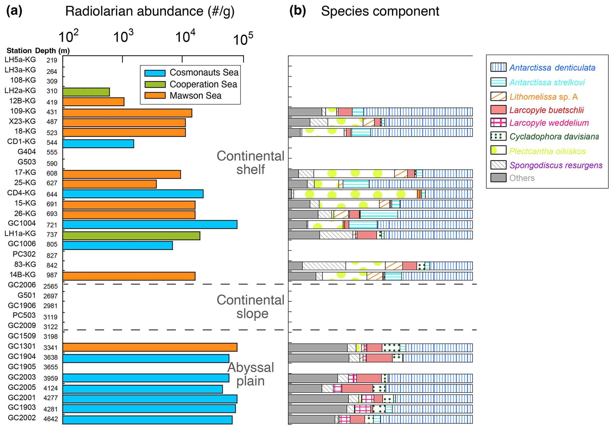
Figure 4 Radiolarian abundance and faunal components of abundant taxa at each site of the surface sediments.

A total of 52 taxa of radiolarians were found in this study (see the Supplement). The number of species tends to be higher on the continental slope and abyssal plain (approximately 35 taxa per sample) than on the continental shelf (around 23 taxa per sample). The most dominant taxa were Antarctissa denticulata, accounting for 29 %–73 % of the total assemblage for each sample, followed by Antarctissa strelkovi (0 %–21 %), Lithomelissa sp. A (0 %–12 %), and Larcopyle buetschlii (0 %–24 %). Figure 4b shows the relative abundance of the above species for each site.

As accompanying radiolarian species, Acanthosphaera spp., Cenosphaera spp., Cycladophora bicornis, Larcopyle nebulum, Larcopyle weddellium, Spongopyle osculosa, and Peripyramis sp. were commonly observed in the abyssal plain. However, their occurrence was limited to the continental shelf (see Supplement data). On the other hand, Cycladophora davisiana, Larcopyle buetschlii, Zygocircus archicircus, Pseudodictyophimus gracilipes, Lithelius minor, Phormospyris stabilis antarctica, Saccospyris antarctica, and Spongotrochus glacialis were common not only in the abyssal plain but also on the continental shelf (see the Supplement). Spongodiscus resurgens, Lithomelissa sp. A, Lithelius nautiloides, and Antarctissa strelkovi were mainly found in the continental shelf samples. Similar radiolarian assemblages observed in this study have been recognized in previous studies in the Southern Ocean (e.g., Petrushevskaya, 1967; Abelmann et al., 1999; Cortese and Prebble, 2015).

Plectacantha oikiskos and Rhizoplegma boreale only appeared in the coastal area. In particular, the abundance of Plectacantha oikiskos is quite conspicuous. Plectacantha oikiskos and Rhizoplegma boreale were observed in coastal areas across the world's oceans, such as in the Norwegian Sea and subarctic Pacific (Jørgensen, 1900, 1905; Bjørklund, 1976; Ikenoue et al., 2012). Furthermore, Nishimura et al. (1997) describe these taxa as coastal area assemblages even in the Southern Ocean. Thus, the results of this study are consistent with previous studies.

4.2.2 Q-mode factor analysis for surface sediments

Q-mode factor analysis is conducted based on 19 samples collected from 431–4642 m water depth and 24 taxa, resulting in the definition of four factors, accounting for about 80 % of the variance of the included fauna (Tables 2 and 3). Figure 5 shows distribution maps of each factor loading in the entire examined area. Figure 6 shows close-up maps of the SC area.

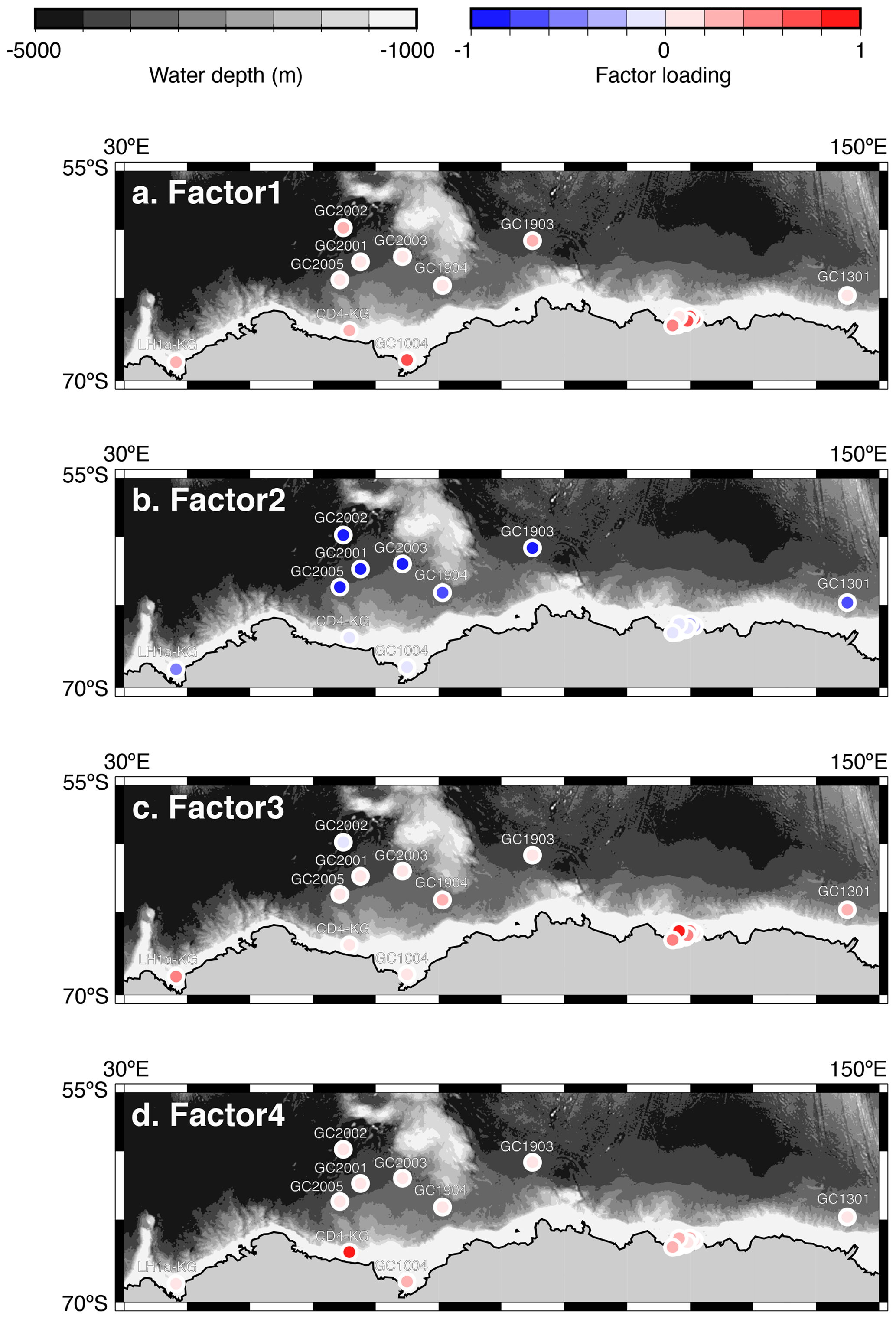
Figure 5 Geographic distribution of factor 1–4 loadings. (a, b, c, d) Geographic distribution of factor loadings of F1, F2, F3, and F4, respectively. The maps (a–d) showing previously published data overlain on the Bedmap2 subglacial topography (Fretwell et al., 2013).

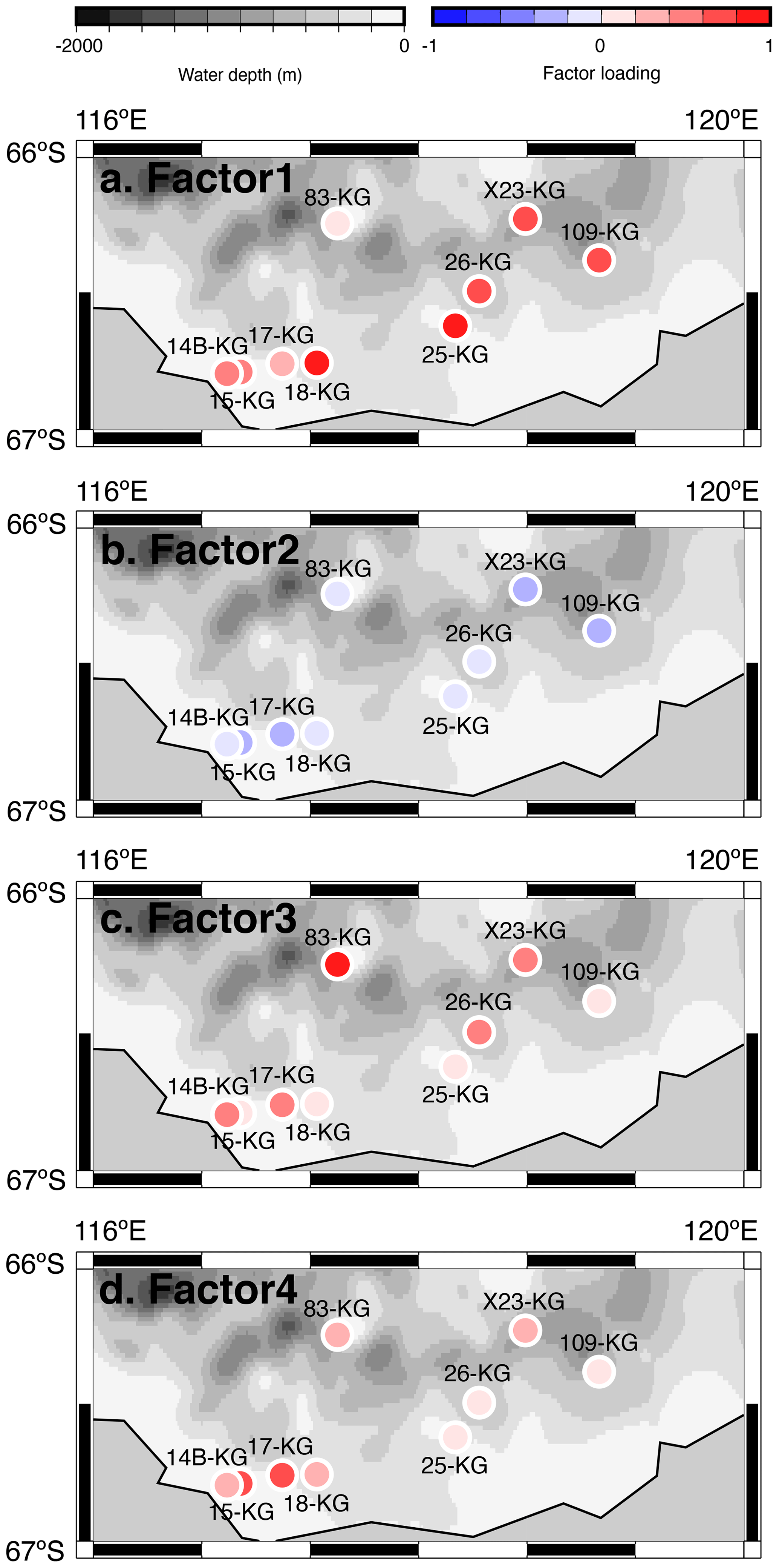
Figure 6 Geographic distribution of factor 1–4 loadings at SC site. (a, b, c, d) Geographic distribution of factor loadings of F1, F2, F3, and F4, respectively, at SC site. The maps (a–d) showing previously published data overlain on the Bedmap2 subglacial topography (Fretwell et al., 2013).

Table 2 Varimax factor matrix.

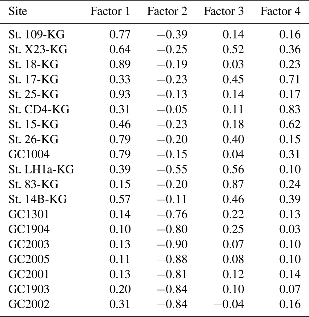
Table 3 Varimax factor score matrix with scaled values. Bold font indicates absolute values greater than 1.

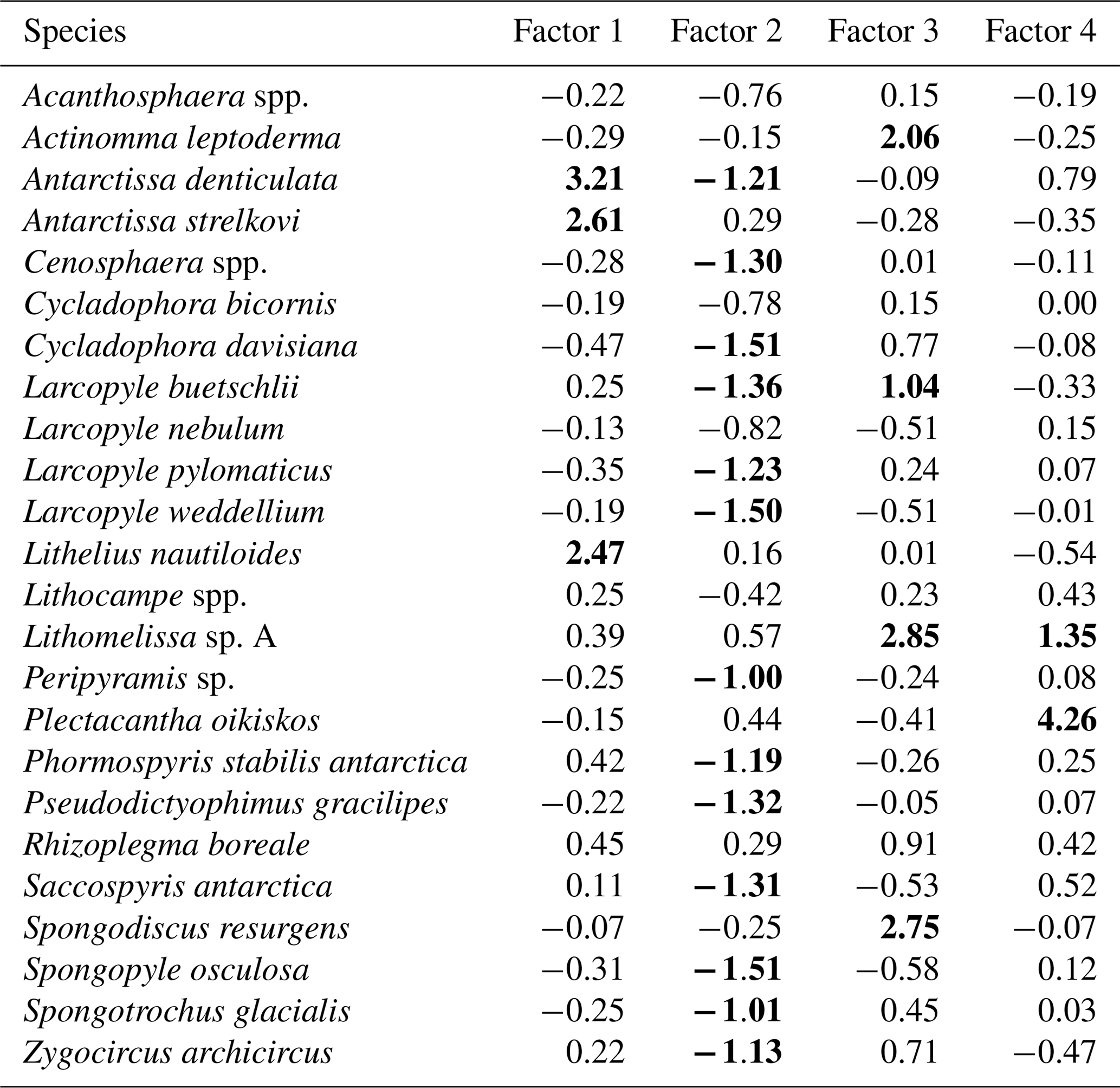
Factor 1 (F1) is the dominant factor, explaining 52 % of the variance in the included fauna. F1 shows factor loadings higher than 0.5 at most continental shelf samples (water depth of 431–987 m) and loading from 0.10 to 0.31 at abyssal plain samples (water depth of 3341–4642 m) (Figs. 5a and 6a; Table 2). In F1, Antarctissa denticulata, Antarctissa strelkovi, and Lithelius nautiloides show high scores (3.21, 2.61, and 2.47, respectively) (Table 3).

Factor 2 (F2) explains 17 % of the variance and shows negative loadings, with less than −0.7 at abyssal plain samples (Figs. 5b and 6b; Table 2). For this factor, 13 taxa exhibit low scores, including Antarctissa denticulata, Cenosphaera spp., Cycladophora davisiana, Larcopyle buetschlii, Larcopyle weddellium, Larcopyle pylomaticus, Peripyramis sp., Phormospyris stabilis antarctica, Pseudodictyophimus gracilipes, Saccospyris antarctica, Spongopyle osculosa, Spongotrochus glacialis, and Zygocircus archicircus (Table 3). In general, negative scores mean the absence of taxa in the corresponding factor. However, due to the negative loadings of F2, negative scores would mean the presence of the corresponding taxa. Therefore, these taxa are present in F2.

Factor 3 (F3) explains 6.6 % of the variance and shows factor loadings higher than 0.5 at continental shelf samples in SC and LHB areas and loadings from −0.04 to 0.25 at abyssal plain samples and continental shelf samples in the Cooperation Sea (Figs. 5c and 6c; Table 2). Values higher than 0.5 are observed at St. X23-KG, St. 83-KG in the SC, and St. LH1a-KG in LHB (Figs. 5c, 6c). For F3, Actinomma leptoderma, Larcopyle buetschlii, Lithomelissa sp. A, and Spongodiscus resurgens show high scores (2.06, 1.04, 2.85, and 2.75, respectively) (Table 3).

Factor 4 (F4) explains 4.2 % of the variance and exhibits high loadings at coastal site samples, particularly at St. CD4-KG off Cape Darnley in the PB area and St. 15-KG and St. 17-KG in the SC area (Figs. 5d and 6d; Table 2). For F4, Plectacantha oikiskos and Lithomelissa sp. A show high scores (4.26, 1.35) (Table 4).

4.3 Plankton tows

4.3.1 Radiolarian abundance and assemblage

Figure 7 shows the living radiolarian abundance at the studied sites. The total abundance of live radiolarians was highest at KC05, the most northerly site, and was 100 times higher at KC05 than at the other sites. Generally, the living radiolarians are not found in the surface layer above 50 m at most sites. The maximum numbers of living radiolarians were recognized at water depths of 50–100 and 100–200 m, with their numbers decreasing with water depth.

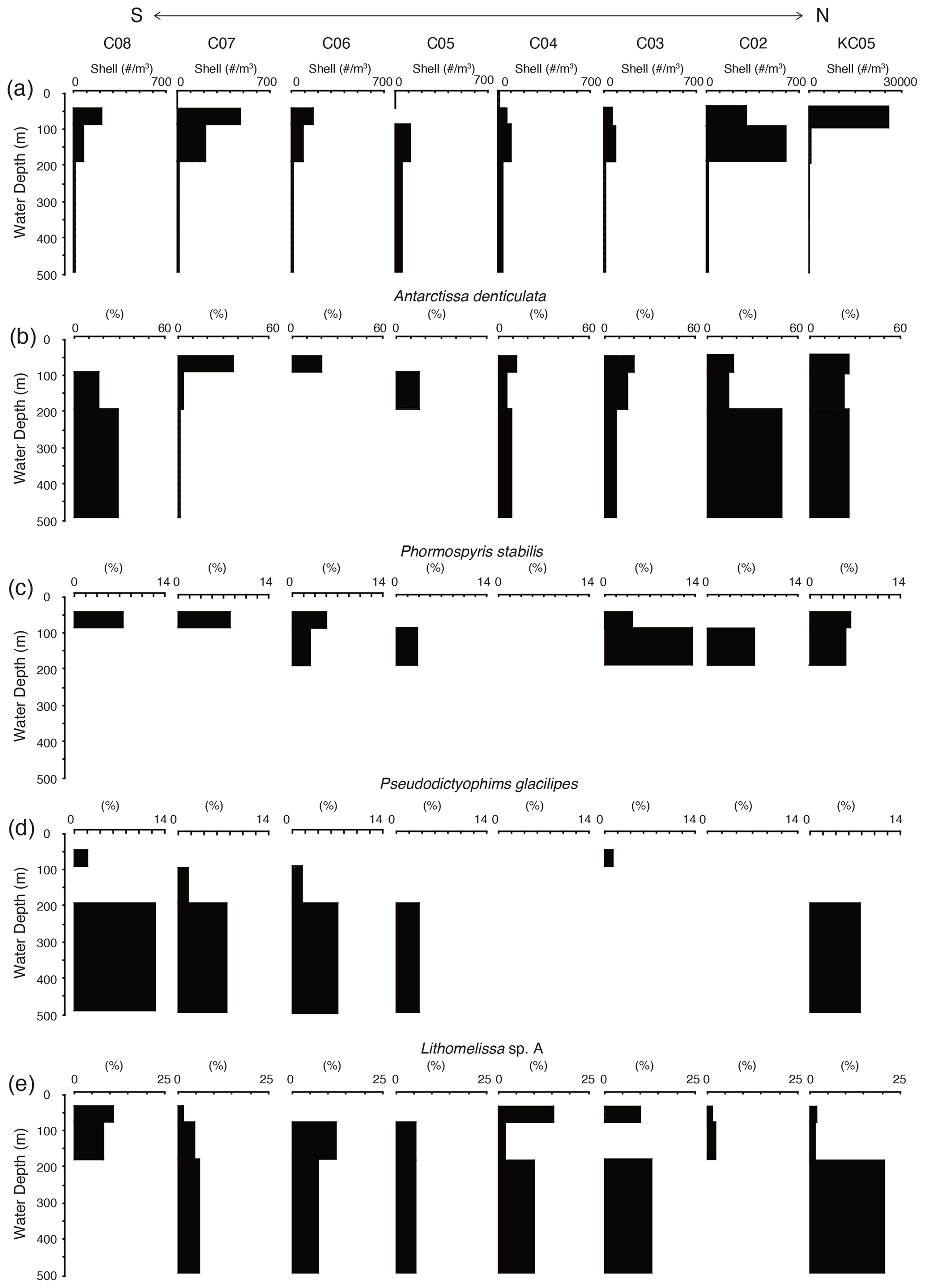
Figure 7 Depth profiles of total living radiolarians and living depth profiles of major radiolarian species from plankton tow samples.

A total of 26 living radiolarian taxa were identified in the plankton samples (see the Supplement). These species are generally found in the Southern Ocean and are similar to the species recognized in surface sediments. Juvenile Antarctissa spp., Antarctissa denticulata, and Lithocampe spp. were the dominant species from the plankton tow samples. Lithocampe spp. were not abundant in the surface sediment samples, but they were abundant in plankton tow samples. Antarctissa denticulata was found from 50 to 500 m, while its juvenile was abundant in the surface layer (50–100 m). This tendency for adults and juveniles to thrive at different depths has also been observed in Larcopyle buetschlii and its juveniles in the Sea of Japan (Itaki, 2016).

4.3.2 Comparison of living and fossil radiolarian assemblages

Of the 19 taxa showing high scores in the Q-mode factor analysis for the surface sediments, 14 taxa were identified, and 5 taxa were absent in the plankton tow samples (Lithelius nautiloides, Larcopyle pylomaticus, Cenosphaera spp., Zygocircus archicircus, and Plectacantha oikiskos). Antarctissa denticulata and Antarctissa strelkovi, showing high scores in F1, were present throughout the surface to subsurface layers in plankton tow samples. Of the taxa having high scores in F2, Phormospyris stabilis antarctica, Saccospyris antarctica, and Spongotrochus glacialis were found in the surface layer (50–100 m) in plankton tow samples. In contrast, Cycladophora davisiana, Larcopyle buetschlii, Larcopyle weddellium, Peripyramis sp., Spongopyle osculosa, Pseudodictyophimus gracilipes, Lithomelissa sp. A, Actinomma leptoderma, and Spongodiscus resurgens, taxa having high scores in F2 and F3, were found in deeper water (100–200 and 200–500 m) in plankton tow samples (Fig. 7; see the Supplement).

5 Discussion

In the Southern Ocean, radiolarian communities have been observed to vary, based on water mass characteristics such as temperature and salinity (e.g., Lowe et al., 2022; Kling, 1979; Kling and Boltovskoy, 1995; Abelmann and Gowing, 1997). Therefore, radiolarian assemblages spanning the water column, from the surface to the bottom, are closely linked to the assemblages in surface sediment depth (Itaki, 2003). In this section, we explored radiolarian assemblages categorized by water mass. We utilized Q-mode factor analysis of surface sediments at different depths and compare them with living radiolarian assemblages observed from plankton tows.

5.1 Continental shelf AASW group (factor 1)

As the result of factor analysis for surface sediments, F1 shows its highest and lowest loadings at continental shelf and abyssal plain samples, respectively (Fig. 5a). Lithelius nautiloides, Antarctissa denticulata, and Antarctissa strelkovi have relatively high scores for this factor (Table 3). Lithelius nautiloides is abundant in surface sediments south of the PF (Hays, 1965; Petrushevskaya, 1971). Antarctissa denticulata is present in surface sediments south of the PF and is more frequent south of SB (Petrushevskaya, 1971). Abelmann et al. (1999) showed that Antarctissa strelkovi has high abundances at 53–58^∘ S and is limited south of the PF in the Weddell Sea (40^∘ W–10^∘ E). In contrast, Petrushevskaya (1971) showed that the abundance of Antarctissa strelkovi in surface sediment samples gradually increases from north to south (data from longitude 10–180^∘ E) (Petrushevskaya, 1971). Dow (1978) concluded that Antarctissa strelkovi is abundant south of the PF, based on factor analysis of the surface sediment (80–110^∘ E). Although the reasons for the regional differences in the distribution of Antarctissa strelkovi are unclear, this species is more abundant in the higher latitudes (continental shelf sites) of our study area (30–150^∘ E). In F1, it was indicated that these three species are related to water conditions south of the SB, which is in agreement with the other abovementioned studies.

In plankton tow data, Antarctissa denticulata and Antarctissa strelkovi were in high abundance in surface-to-subsurface water (50–100, 100–200, and 200–500 m), showing that these two species live in the surface water south of the PF (Fig. 7; see the Supplement). Previous studies from plankton tow also show that three of the species having high scores in F1 in our data from Q-mode factor analysis of surface sediments (Antarctissa denticulata, Antarctissa strelkovi, and Lithelius nautiloides) dominantly occur in surface water (∼ 200 m) south of the PF (Morley and Stepien, 1985). The cold water cooled by meltwater from ice sheets and sea ice is located in the nearshore AASW (Fig. 2), indicating that Antarctissa denticulata, Antarctissa strelkovi, and Lithelius nautiloides inhabit the nearshore AASW, which is even colder than offshore AASW.

5.2 Offshore AASW and CDW groups (factor 2)

The result of Q-mode factor analysis from surface sediments shows high and low loadings in the abyssal plain and continental shelf samples, respectively (Figs. 5b and 6b; Table 2), suggesting that the taxa showing high scores in F2 live in the open ocean north of SB. The AASW, CDW, and AABW are located offshore (Fig. 2), but because waters rich in radiolarian are generally limited to ocean depths shallower than 1000 m (Boltovskoy, 2017), the AABW, which is located in lower layers, is thought to have few radiolarian species. Thus, the 13 taxa displaying relatively high scores in F2 (>1.0) could be living in the offshore AASW or CDW.

5.2.1 Offshore AASW group

Of the species showing high scores in F2, Antarctissa denticulata, Phormospyris stabilis antarctica, Spongotrochus glacialis, and Saccospyris antarctica were recognized in the surface water (50–100 m) from plankton tow samples (Fig. 7; see the Supplement data). Moreover, previous studies of plankton tows and surface sediments show that these taxa are observed north of SB (Morley and Stepien, 1985; Abelmann and Gowing, 1997; Abelmann et al., 1999). Therefore, these taxa are likely to live in offshore AASW in the Southern Ocean. All of these taxa are different from the taxa showing high scores in F1, except for Antarctissa denticulata. This suggests that the radiolarian assemblage differs between nearshore and offshore.

Antarctissa denticulata reaches a high score (>1.0) in two factors (F1 and F2). The other two species (Antarctissa strelkovi and Lithelius nautiloides) that had high scores in F1 only are highly abundant in the nearshore, while Antarctissa denticulata is in a wider region (south of 50^∘ S) compared to these two species (Abelmann et al., 1999; Hays, 1965). Therefore, it is suggested that Antarctissa denticulata shows a high score not only in F1 (continental shelf) but also in F2 (abyssal plain), which is the offshore factor.

5.2.2 CDW group

Of the nine taxa showing high scores in F2 from Q-mode factor analysis from surface sediments, six taxa could not be associated with the surface layer (Cycladophora davisiana, Larcopyle buetschlii, Larcopyle weddellium, Peripyramis sp., Pseudodictyophimus gracilipes, and Spongopyle osculosa) that increased with depth, and these taxa were most abundant in 200–500 m from plankton tow samples (Fig. 7; see the Supplement). Previous studies report that Larcopyle pylomaticus, Larcopyle weddellium, Spongopyle osculosa, and Cycladophora davisiana are also observed below a water depth of 200 m from plankton tows in the Southern Ocean (Morley and Stepien, 1985). The habitat depth of Larcopyle buetschlii differs between juveniles and adults in the Japan Sea, where the adult forms are abundant between 200 and 1000 m water depth. In contrast, the juvenile Larcopyle buetschlii is restricted to shallow water above 200 m (Itaki, 2016). Most of the Larcopyle buetschlii specimens observed in this study are adults; hence, they most likely represent forms that live in deeper habitats. Although the ecological information on Zygocircus archicircus is uncertain, Zygocircus group is recognized in surface sediment and sediment trap samples in the oceans worldwide (e.g., Abelmann et al., 1999; Boltovskoy and Riedel, 1980; Renz, 1976) and is reported to live in the mesopelagic zone in the North Pacific Ocean (Okazaki et al., 2004; Kling and Boltovskoy, 1995). The habitat depth of Zygocircus archicircus in the Southern Ocean is still unknown; however, if these taxa showing high scores in F2 have similar habitat depths in the Southern Ocean, then they can be identified as species that dwell in the mesopelagic zone. Although the habitat depth of Cenosphaera spp. has been unclear, they are also likely to inhabit the mesopelagic zone of the Southern Ocean because they have not been found in the plankton tows from the surface layer of the Southern Ocean.

Thus, nine taxa showing high scores in F2 are suggested to dwell in deep water, indicating that they also dwell in CDW, warm deep water, to the south of 60^∘ in the Southern Ocean. This result is also supported by a previous study on the horizontal and vertical distributions of living polycystine radiolarian taxa on a N–S transect (30–58^∘ S) (Abelmann and Gowing, 1997), in which Cycladophora davisiana, Larcopyle pylomaticus, Larcopyle weddellium, Pseudodictyophimus gracilipes, and Spongopyle osculosa are shown to be closely related to the CDW factor (below 400 m), based on the Q-mode factor analysis.

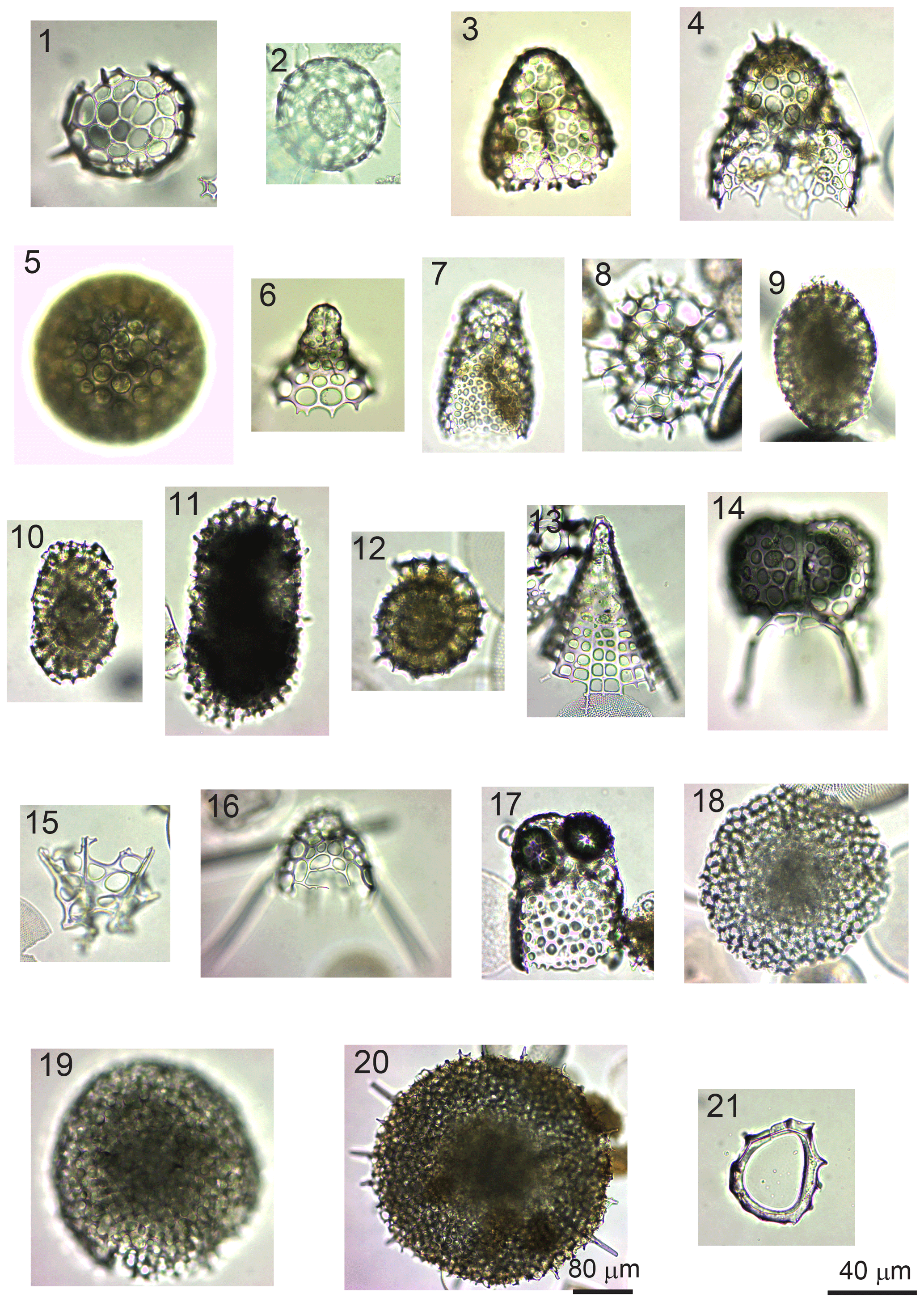
Figure 8 (1) Acanthosphaera spp. (sample GC1904). (2) Actinomma leptoderma (Jørgensen) (GC1904). (3) Antarctissa denticulata (Ehrenberg) (GC1904). (4) Antarctissa strelkovi (Petrushevskaya( (14B-KG). (5) Cenosphaera spp. (GC1904). (6) Cycladophora davisiana (Ehrenberg) (GC1904). (7) Lithomelissa sp. A (C2002). (8) Larcopyle buetschlii (Dreyer) (GC1904) (juvenile). (9) Larcopyle buetschlii (Dreyer) (14B-KG) (adult). (10) Larcopyle weddellium (Lazarus, Faust, and Popova-Goll) (GC1904). (11) Larcopyle pylomaticus (Riedel) (GC1904). (12) Lithelius nautiloides (Popofsky) (14B-KG). (13) Peripyramis sp. (GC2002). (14) Phormospyris stabilis (Goll) antarctica (Haecker) (GC2002). (15) Plectacantha oikiskos (Jørgensen) (14B-KG). (16) Pseudodictyophimus gracilipes (Bailey) (GC2002). (17) Saccospyris antarctica (Haecker) (GC1904). (18) Spongodiscus resurgens (Ehrenberg) (12B-KG). (19) Spongopyle osculosa (Dreyer) (GC2002). (20) Spongotrochus glacialis (Popofsky) (14B-KG). (21) Zygocircus productus (Popofsky) (GC1904). The 40 µm scale bar applies to samples (1)–(19) and (21), while the 80 µm scale bar applies to sample (20).

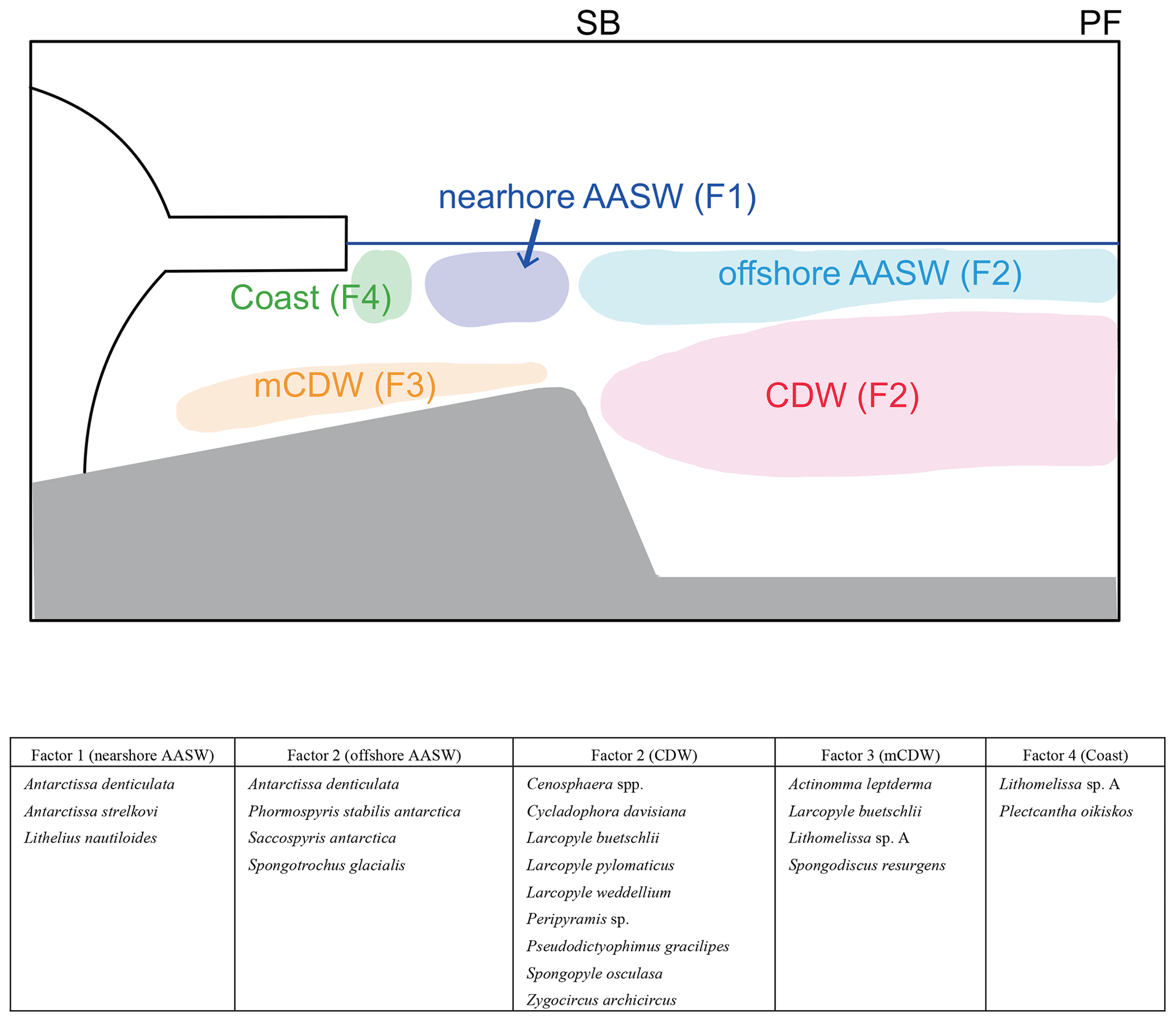
Figure 9 Schematic figures showing typical radiolarian assemblages and their relation to water masses. In this study area, the major fronts are the polar front (PF) and southern boundary of Antarctic Circumpolar Current (SB). The major water masses are Antarctic Surface Water (AASW), Circumpolar Deep Water (CDW), and modified CDW (mCDW).

5.3 mCDW group (factor 3)

F3 shows high loadings at continental shelf samples in SC and LHB and low loadings at the continental shelf in PB and abyssal plain samples (Figs. 5c and 6c). For this factor, Larcopyle buetschlii, Lithomelissa sp. A, Actinomma leptoderma, and Spongodiscus resurgens show high scores (1.04, 2.85, 2.06, and 2.75). Our plankton tow data suggest that these taxa were found in shallow and deep waters and were abundant in 200–500 m (Fig. 7; see the Supplement). As mentioned above, Larcopyle buetschlii (adult) dwells in deep water, and it was identified as a species that dwells in the mesopelagic zone. Actinomma leptoderma has been reported in high-latitude oceans, such as the Arctic Ocean and Greenland Sea (Hülsemann, 1963; Tibbs, 1967; Petrushevskaya, 1969), and observed in the relatively warm mesopelagic zone (Jørgensen, 1905). It has been reported that Lithomelissa sp. A dwells in the mesopelagic zone in the Southern Ocean (∼ 55^∘ S) from factor analysis of plankton tow data (Abelmann and Gowing, 1997). These insights suggest that these taxa inhabit relatively deep waters.

High loadings in F3 were found at St. 83-KG, St. X23-KG, and LH1a-KG (0.87, 0.52, and 0.56, respectively). The vertical profiles of temperature and salinity suggest the intrusion of mCDW onto these sites (Fig. 3; see the Supplement). Therefore, if these taxa showing high scores in F3 also live to the south of SB in the deep ocean, then they can be identified as mCDW taxa. However, plankton tow data at the continental shelf are required to further understand the habitat depth of this species south of 65^∘ S.

5.4 Coastal group

F4 shows the highest loadings in coastal samples (St.14B-KG, St. 15-KG, St. 12B-KG, St. 17-KG, and CD4-KG). Moreover, Plectacantha oikiskos and Lithomelissa sp. A. Plectacantha oikiskos, showing high scores in F4, have been observed in coastal areas at high latitudes, such as fjords of the Norwegian Sea, Southern Ocean (e.g., Jørgensen, 1905; Nishimura et al., 1997), and are reported to be common in the plankton at the ice edge in the Greenland Sea (Swanberg and Eide, 1992). Lithomelissa sp. A was abundant in the coastal area in the Southern Ocean (Petrushevskaya, 1967).

The sites with high loadings in F4 (St. 14B-KG, St. 15-KG, St. 12B-KG, St. 17-KG, and CD4-KG) were located near polynya and the edge of glacier areas, suggesting that these taxa showing high scores in F4 (Plectacantha oikiskos and Lithomelissa sp. A) may be related to the ice edge. Lithomelissa sp. A exhibited high loadings in both F3 and F4 and may be influenced by the ice edge environment, as well as the water masses.

6 Conclusion

For the first time, this study provided a radiolarian assemblage dataset from the continental shelf to the abyssal plain of the Southern Ocean (south of the PF), based on the analysis of surface sediment and plankton tow samples. The abundance and diversity of radiolarians in surface sediments in the Southern Ocean (south of PF) increase with water depth and can be related to different water masses.

The four factors (F1–F4) related to the hydrographic conditions were found through Q-mode factor analysis of the radiolarian dataset for 24 species and species groups at 19 surface sediments sites (Fig. 9). F1 shows high loadings at continental shelf sites, suggesting that its characteristic taxa inhabit nearshore AASW and are affected by ice sheet and sea ice melting water. F2 shows high loading on the abyssal plain sites, suggesting that taxa associated with F2 inhabit the north of SB. Comparison with plankton tow data suggested that F2 taxa dwell in the CDW or offshore AASW (Fig. 9). F3 reaches high loadings at the continental shelf sites (St. 83-KG, St. X23-KG, and LH1a-KG), where mCDW intrudes onto the continental shelf, suggesting that this assemblage lives in the mCDW. F4 has high loadings in the coastal area (ice edge areas), suggesting that this assemblage dwells near ice edge areas.

This study provides information on radiolarian assemblages and how they relate to hydrographic conditions. However, it is difficult to use sediment data as direct evidence for the depth distribution of radiolarians in the Southern Ocean south of SB. Hence, it is crucial to accurately identify the habitat depth using plankton tow experiments in the Southern Ocean south of SB in the future.