Recent benthic foraminifera communities offshore of Thwaites Glacier in the Amundsen Sea, Antarctica: implications for interpretations of fossil assemblages

Benthic foraminiferal assemblages are useful tools for paleoenvironmental studies but rely on the calibration of live populations to modern environmental conditions to allow interpretation of this proxy downcore. In regions such as the region offshore of Thwaites Glacier, where relatively warm Circumpolar Deep Water is driving melt at the glacier margin, it is especially important to have calibrated tracers of different environmental settings. However, Thwaites Glacier is difficult to access, and therefore there is a paucity of data on foraminiferal populations. In sediment samples with in situ bottom-water data collected during the austral summer of 2019, we find two live foraminiferal populations, which we refer to as the Epistominella cf. exigua population and the Miliammina arenacea population, which appear to be controlled by oceanographic and sea ice conditions. Furthermore, we examined the total foraminiferal assemblage (i.e., living plus dead) and found that the presence of Circumpolar Deep Water apparently influences the calcite compensation depth. We also find signals of retreat of the Thwaites Glacier Tongue from the low proportion of live foraminifera in the total assemblages closest to the ice margin. The combined live and dead foraminiferal assemblages, along with their environmental conditions and calcite preservation potential, provide a critical tool for reconstructing paleoenvironmental changes in ice-proximal settings.

1 Introduction

The ice loss from the rapidly thinning and retreating Thwaites and Pine Island glaciers of the West Antarctic Ice Sheet (WAIS) in the Amundsen Sea is contributing significantly to global sea level rise and is threatening the stability of this ice sheet (Joughin et al., 2014; Rignot et al., 2013, 2019; Milillo et al., 2019). Marine geologic data have revealed the history of ice sheet retreat in the Amundsen Sea, with deglaciation in the west starting as early as 22.4 calibrated kiloyears Before Present (cal ka BP; Smith et al., 2011; Larter et al., 2014) and 16.4 cal ka BP in the east (Kirshner et al., 2012). The grounding zones of both Thwaites and Pine Island glaciers retreated to within ∼ 100 km of their present-day positions by 10 cal ka BP (Fig. 1a; Hillenbrand et al., 2013; Larter et al., 2014). The ice sheet is assumed to have remained largely stable during the past 10 cal ka, as suggested by regional sea level data that imply relatively small-scale changes (Braddock et al., 2022). However, a temporary grounding zone retreat upstream of its modern position at some point during the Holocene was inferred from a phase of ice sheet surface lowering below the present altitude further inland (Balco et al., 2023).

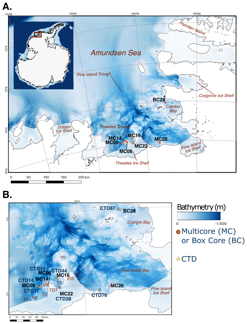
Figure 1 Bathymetric maps of the Amundsen Sea with coastlines and ice shelf margins marked by black lines (Hogan et al., 2020). (a) Locations of investigated NBP19-02 multicores and box cores (filled orange circles). (b) Detailed map offshore from the Thwaites Glacier Tongue (TGT), Eastern Ice Shelf (EIS), and Pine Island Bay, showing locations of studied cores (filled orange circles) and associated conductivity, temperature, and depth (CTD) measurements (filled yellow triangles). H1 and H2 are bathymetric highs; T2, T3, and T4 are bathymetric troughs (see Wåhlin et al., 2021).

The modern retreat of the Pine Island Glacier (Smith et al., 2017) and Thwaites Glacier (Clark et al., 2024) is thought to have started in the 1940s, possibly in response to sustained tropical forcing. Ocean modeling suggests that while this natural climate variability drove the initial grounding zone retreat, it was likely sustained by increasing anthropogenic forcing (Holland et al., 2019). However, the main driver of the retreat is the sub-ice-shelf melt from the relatively warm Circumpolar Deep Water (CDW; Jenkins et al., 2010; Jacobs et al., 2012; Wåhlin et al., 2021). There is evidence that CDW also influenced ice melting during the Holocene (Hillenbrand et al., 2017). Despite the improved understanding of the timing of grounding zone retreat, the historic drivers of change remain relatively poorly constrained.

In other areas of Antarctica, benthic foraminiferal assemblages have been calibrated to environmental conditions (e.g., Ishman and Domack, 1994; Majewski, 2005), and those calibrations have been applied in other areas to allow this proxy to be interpreted downcore in the paleorecord (Majewski et al., 2016; Totten et al., 2017; Seidenstein et al., 2024). To strengthen the use of benthic foraminiferal assemblages as a proxy, the ecologic affinities of foraminifera must be determined. A “foraminiferal population” is defined in this paper as the total living census at one point in time, and a “foraminiferal assemblage” is defined as the preserved census averaged over a period of time (e.g., Echols, 1971).

While there are detailed modern foraminiferal assemblage studies for several regions around Antarctica, including the Antarctic Peninsula (Ishman and Domack, 1994; Jones and Pudsey, 1994; Ishman and Szymcek, 2003; Majewski, 2010; Rodrigues et al., 2015; Majewski et al., 2016), the Ross Sea (Osterman and Kellogg, 1979; Bernhard, 1987; Ward et al., 1987; Violanti, 1996, 2000; Pawlowski et al., 2007; Capotondi et al., 2018, 2020), and the Weddell Sea (Anderson, 1975; Mackensen et al., 1990; Cornelius and Gooday, 2004; Pawlowski et al., 2007), there is a dearth of modern population data from the Amundsen Sea (Pflum, 1966; Kellogg and Kellogg, 1987; Majewski, 2013). Without modern population data, the interpretations of fossil benthic foraminiferal assemblages in the paleo-record are limited.

Here, we investigated seven seafloor surface sediment samples from the Amundsen Sea shelf for live (i.e., stained) and dead (i.e., unstained) foraminifera to help develop a proxy for reconstructing past environmental conditions in the area.

1.1 Oceanographic setting

The Amundsen Sea is located on the West Antarctic continental margin in the southeastern Pacific sector of the Southern Ocean. The study area comprises the inner continental shelf of the eastern Amundsen Sea Embayment, including the area proximal to the Thwaites Glacier ice front (Fig. 1). The seafloor of the continental shelf is characterized by bathymetric troughs that act as cross-shelf pathways for CDW, and water depths on the inner shelf can reach over 1200 m (Fig. 1; Jacobs et al., 1996; Nitsche et al., 2007; Jenkins et al., 2010; Rignot et al., 2013; Hogan et al., 2020).

Table 1 In situ hydrographic conditions, averaged from the deepest 5 m interval of conductivity, temperature, and depth (CTD) casts closest to studied surface sediment sample sites. Sea ice cover was averaged for the austral summers (December–February) from 2014–2019. DO is for the dissolved O₂ concentration.

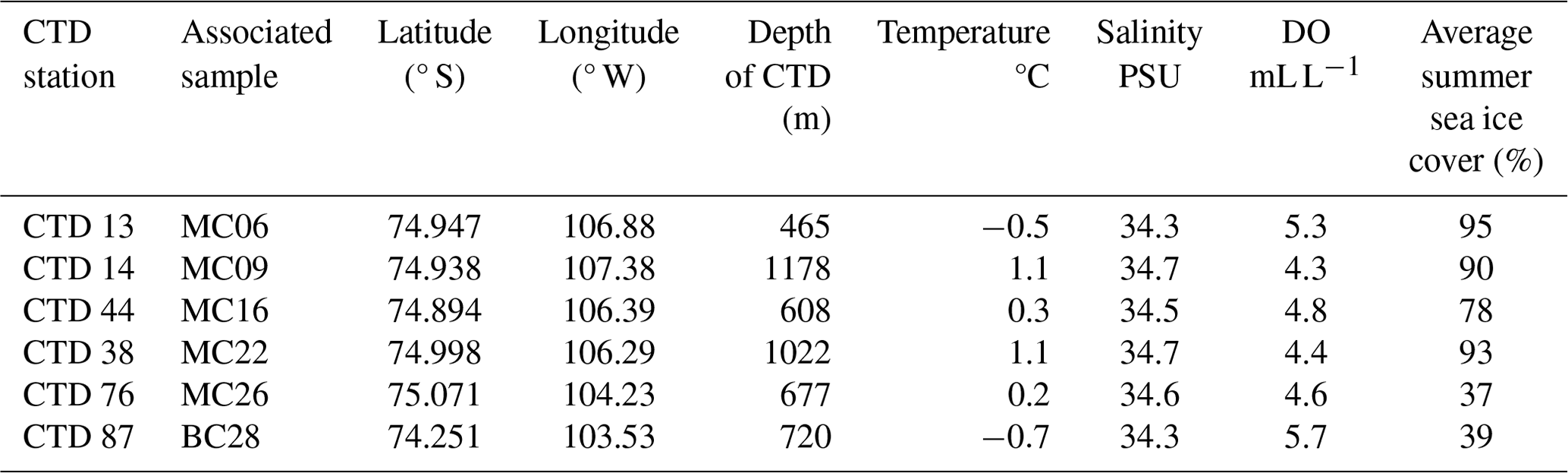
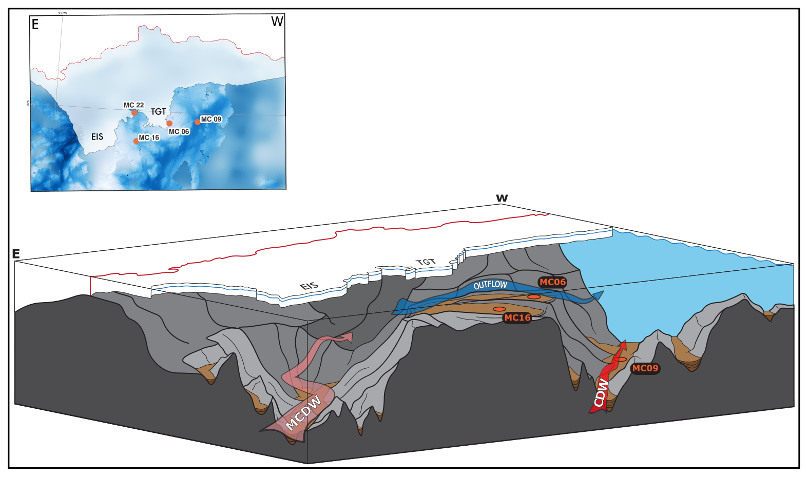
Figure 2 Map view (above) and perspective view from NE (below) of investigated core sites directly offshore from EIS and TGT. Site MC22 is not visible in the perspective view as it lies to the southwest of the bathymetric high, H1. Bathymetry is from Hogan et al. (2020). Based on Wåhlin et al. (2021), water masses are represented by arrows. The red arrow represents relatively warm and saline Circumpolar Deep Water (CDW); the blue arrow represents the relatively cooler, fresher, and glacial-melt-influenced outflow; and the pink arrow possibly represents modified CDW.

The CDW present on the Amundsen Sea continental shelf is typically modified compared to “pure” CDW found seaward of the continental shelf (e.g., Wåhlin et al., 2010) due to both the mixing with Antarctic Surface Water and with glacial meltwater. In this paper, we refer to all varieties of relatively warm deep water as “CDW”. At the Thwaites Glacier ice shelf front, CDW at a water depth below 800 m has a temperature of 1.0 °C, a salinity of 34.7 PSU (practical salinity units), and a dissolved oxygen (DO) concentration of ca. 4.3 mL L⁻¹ (sites MC09 and MC22 in Table 1; Wåhlin et al., 2021). The CDW flows across the continental shelf through Pine Island Trough, reaching the grounding zone of the Pine Island Glacier, where it causes significant sub-ice-shelf melting (Dutrieux et al., 2014). The resulting glacial meltwater mixes with CDW and flows westward beneath the Thwaites Eastern Ice Shelf (EIS) and Thwaites Glacier Tongue (TGT) (Fig. 1; Wåhlin et al., 2021). Autonomous underwater vehicle (AUV) data confirm that CDW also flows southward in a small bathymetric trough located between the EIS and the TGT (“T3” in Wåhlin et al., 2021; Fig. 1a). There is no evidence of glacial meltwater in trough T3, indicating the direct inflow of relatively unmodified CDW to the front of the ice shelf (Fig. 2; Wåhlin et al., 2021).

The glaciers draining into the Amundsen Sea Embayment contribute fresh water to the ocean not only through sub-ice-shelf melting but also grounding zone discharge of subglacial meltwater (Hager et al., 2022; Lepp et al., 2022). Entrained in the subglacial meltwater are fine detrital particles, providing nutrients for planktic organisms. After death, the planktic organisms become food for benthic communities (e.g., Fragoso, 2009; Arrigo et al., 2012; Gerringa et al., 2012; Vick-Majors et al., 2020). More nutrients are brought onto the continental shelf entrained in CDW (St-Laurent et al., 2019). Another important, but limited, nutrient for planktic and benthic organisms in the Southern Ocean is iron (e.g., Arrigo et al., 2012). Weathering of volcanogenic sediments near the Pine Island Glacier is thought to be one mechanism that releases iron into the system, which may facilitate higher primary productivity (Herbert et al., 2023).

Polynyas are areas of open water that form seasonally or exist all year round. In seasonal polynyas, phytoplankton blooms occur in the spring and summer when sunlight is not blocked by ice. Just like other planktic organisms, phytoplankton becomes food for benthic communities after death. The largest and most productive polynya in the Southern Ocean is the Amundsen Sea Polynya offshore from the Dotson Ice Shelf in the western Amundsen Sea Embayment (Fig. 1; Arrigo et al., 2015). The Pine Island Polynya (PIP), in the easternmost Amundsen Sea, can extend northward beyond Cranton Bay (Fig. 1). Though PIP does not form annually, it does reoccur often (Stammerjohn et al., 2015; Herbert et al., 2023). In this study, two of the sample sites are located in PIP and thus have high seasonal variability in sea ice cover (Fig. 1b). The other study sites lie under more extensive sea ice cover, even during austral summers.

1.2 Previous benthic foraminiferal studies from the WAIS

In an Antarctic-wide study, Mikhalevich (2004) concluded that the seafloor substrate and the prevailing oceanographic conditions are the main controls for epi- and infaunal shelf foraminifera. Substrates with coarse-grained unsorted sediments without freshwater influence are characterized by a relatively high abundance of benthic foraminiferal specimens and high foraminiferal species diversity (Mikhalevich, 2004). On the West Antarctic continental shelf in the eastern Pacific sector, a relationship between the presence of CDW and benthic foraminiferal assemblages in seafloor sediments has been reported (Ishman and Domack, 1994; Majewski, 2013).

Only three studies investigating modern benthic foraminiferal assemblages in core-top sediments from the Amundsen Sea continental shelf and slope have been published (Pflum, 1966; Kellogg and Kellogg, 1987; Majewski, 2013). However, either the samples were not stained, and the benthic foraminiferal assemblages were not analyzed quantitatively (Pflum, 1966; Kellogg and Kellogg, 1987), or the samples were stained, but only dead benthic foraminifera were encountered (Majewski, 2013). Kellogg and Kellogg (1987) investigated core-top sediments from the continental shelf in the eastern Amundsen Sea Embayment, including Pine Island Bay (Fig. 1). The authors observed high concentrations of calcareous benthic foraminifera on the outer continental shelf north of King Peninsula, the lowest concentration of benthic foraminifera in Pine Island Bay, and high concentrations of diatoms and agglutinated foraminifera along the eastern Amundsen Sea Embayment coast between Pine Island Bay and King Peninsula (Fig. 1a; Kellogg and Kellogg, 1987). The high concentrations of diatoms and agglutinated foraminifera along the eastern embayment coast were attributed to high plankton productivity within polynyas and increased calcite dissolution in oxygen-depleted bottom waters at water depths below 500 m (Kellogg and Kellogg, 1987).

In a more recent study of Pine Island Trough (Fig. 1), Kasten core-top sediments were treated with rose bengal, but no stained foraminifera were observed (Majewski, 2013). The lack of living tissue in the benthic foraminiferal tests was attributed to the loss of the typically very “soupy” seafloor surface sediments during the recovery of the Kasten cores or, at a few sites, seafloor disturbance by iceberg plowing (Majewski, 2013). Thus, the foraminiferal assemblages described were considered “dead” (Majewski, 2013). The two key environmental parameters determined by Majewski (2013) to control the benthic foraminifera identified in the >125 and 63–125 µm size fractions are water mass distribution (i.e., CDW influence) and, at greater water depths, the local calcite compensation depth (CCD). Within the 63–125 µm size fraction, three major foraminiferal assemblages (FAs) were identified: the Epistominella spp. FA, the Portatrochamina spp. FA (including the accessory species Adercotryma glomerata and Spiroplectammina biformis), and the Pseudobolivina antarctica FA (including the accessory of Adercotryma glomerata but excluding any Portatrochammina spp.).

On the western Antarctic Peninsula continental shelf, two benthic foraminiferal assemblages have been linked to specific water masses (Ishman and Domack, 1994). Areas of seafloor with overlying CDW were characterized by a Bulimina aculeata FA, while areas of seafloor with overlying cooler and less saline Weddell Sea Transitional Water were typified by a Fursenkoina spp. FA (Ishman and Domack, 1994). Following this work on modern foraminiferal assemblages from the western Antarctic Peninsula shelf (Ishman and Domack, 1994), B. aculeata was considered an indicator species for CDW influence in the Amundsen Sea Embayment (Majewski, 2013).

B. aculeata was identified in early- to mid-Holocene sediments from Ferrero Bay at the eastern Amundsen Sea coast, indicating that the CDW influenced glacial retreat in Ferrero Bay during that time (Totten et al., 2017). Other indicators of CDW may include the calcareous benthic foraminifera Globocassidulina subglobosa and Nonionella spp. They were reported from early-Holocene sediments in Pine Island Bay, which were deposited under strong CDW influence as inferred from trace metal and stable carbon isotope data of benthic foraminiferal tests (Hillenbrand et al., 2017). The G. subglobosa and Nonionella spp. were also associated with the presence of an ice shelf (Hillenbrand et al., 2017), but we speculate that they alternatively may signify a stronger CDW influence. More data on live foraminiferal populations and their environmental conditions are required to improve interpretations of fossil assemblages in the Amundsen Sea Embayment.

2 Methods

From January to March 2019 on expedition NBP19-02 in the Amundsen Sea Embayment, bathymetric data, hydrographic data, and sediment cores were collected on research vessel/icebreaker (RV/IB) Nathaniel B. Palmer (NBP) by the Thwaites Offshore Research (THOR) and Thwaites–Amundsen Regional Survey and Network (TARSAN) Integrating Atmosphere–Ice–Ocean Processes affecting the Sub-Ice-Shelf Environment projects of the International Thwaites Glacier Collaboration (ITGC). All data and samples presented in this paper were collected during that cruise (Larter et al., 2020).

2.1 Hydrographic measurements and sea ice conditions

Sea-Bird CTD casts measured seawater properties at or near each seafloor surface sampling site (Table 1). The Sea-Bird CTD was equipped with temperature, conductivity, dissolved oxygen, and pressure sensors. The hydrographic data averaged from the deepest 5 m of the CTD cast (or the 5 m average at the water depth of the core site if the CTD location was slightly offset from this site) were averaged to gain an understanding of the bottom-water conditions affecting the benthic foraminiferal community in the seafloor surface sediments.

We estimate the mean sea ice cover at each core site for 4 years, as this represents the likely maximum lifespan of benthic foraminifera (Table 1; e.g., Hayward et al., 2014; Hohenegger, 2018). The sea ice cover was estimated using version V0.9.2 of the ARTIST Sea Ice (ASI) sea ice concentration product from the University of Bremen, with the dataset gridded at 3.125 km spacing (Spreen et al., 2008). For each core site, we extracted the average percentage of sea ice cover for the corresponding 3.125 km ×3.125 km grid cell. Subsequently, the daily measurements of austral summers (December to February) from 2015 to 2019 CE were averaged (Table 1). In this paper, we refer to these sea ice cover estimates as “summer sea ice cover”.

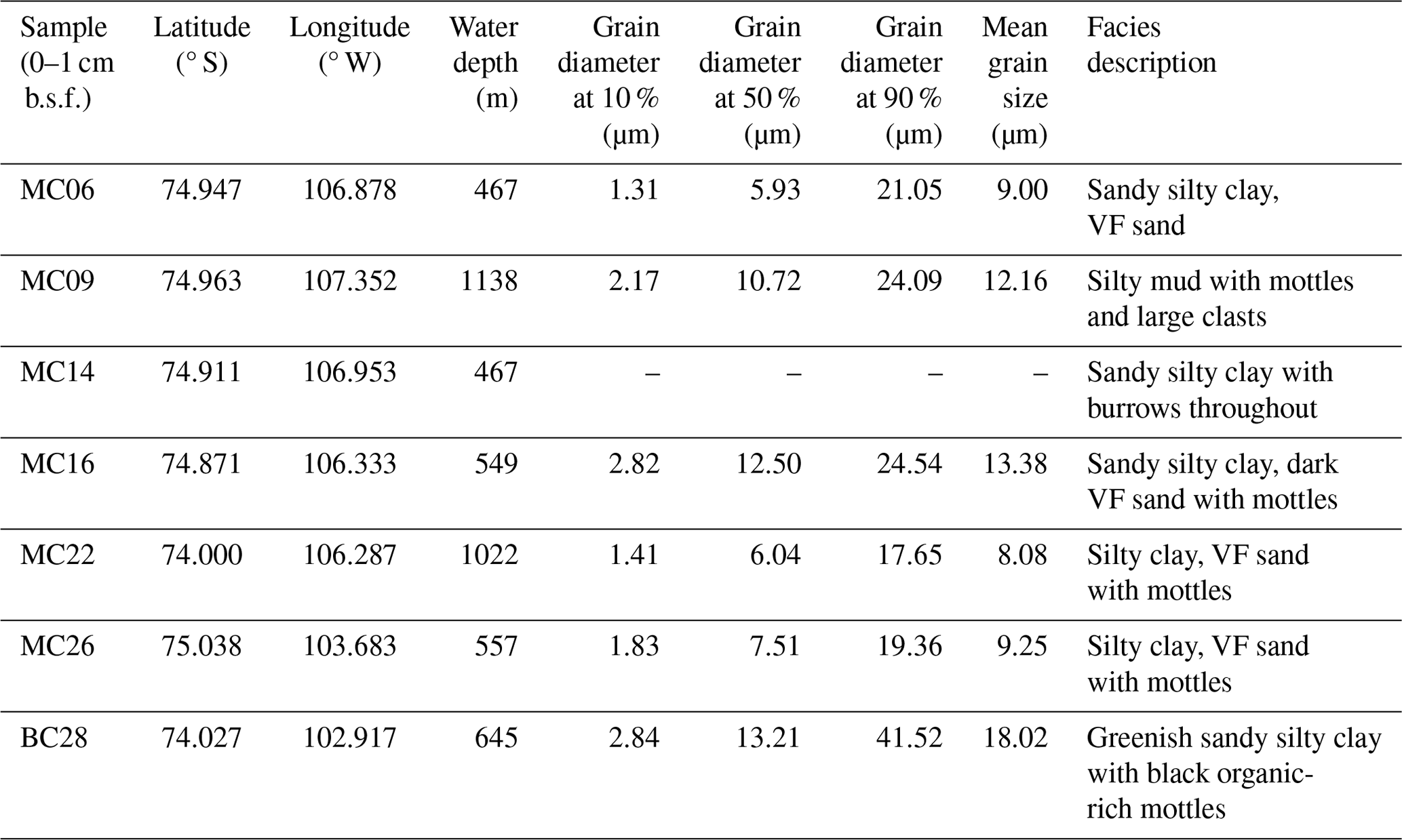
Table 2 NBP19-02 multicore locations and substrate properties (VF is for very fine).

2.2 Core material

Core locations were chosen based on sea ice conditions and acoustic sub-bottom profiles (Knudsen; Chirp 3260; 3.5 kHz) collected during NBP19-02 (Table 2; Figs. 1 and S1 in the Supplement). An Ocean Scientific International Ltd multicorer (MC) was deployed to recover undisturbed surface sediments with the seafloor–seawater interface well preserved. The MC is equipped with 12 individual sampling tubes of 11 cm diameter, from which sub-core slices were extracted. Each sub-core selected for the foraminiferal analysis was placed vertically on an extruding device, as a piston incrementally extruded the sediment cores. Sediment slices of 1 cm, with approximately 95 cc of sediment, were cut from the extruded material and either immediately processed (see Sect. 2.3) or placed in sample bags.

An Ocean Instruments BX-650 giant box corer (BC) was deployed at site BC28 (Fig. 1). The BC also preserves the seafloor–seawater interface. BCs were sub-sampled by pushing polycarbonate MC core tubes into the recovered sediment and then extruding them into sub-core slices following the procedures for the MCs. Archives of a few of the NBP19-02 MC and BC cores, as duplicates collected from the same cores, are stored at the Marine and Geology Repository of Oregon State University (OSU-MGR) in Corvallis, Oregon, USA.

In this study, we analyzed benthic foraminifera (if present) in seafloor surface sediment samples (0–1 cm depth) of six MCs and one BC.

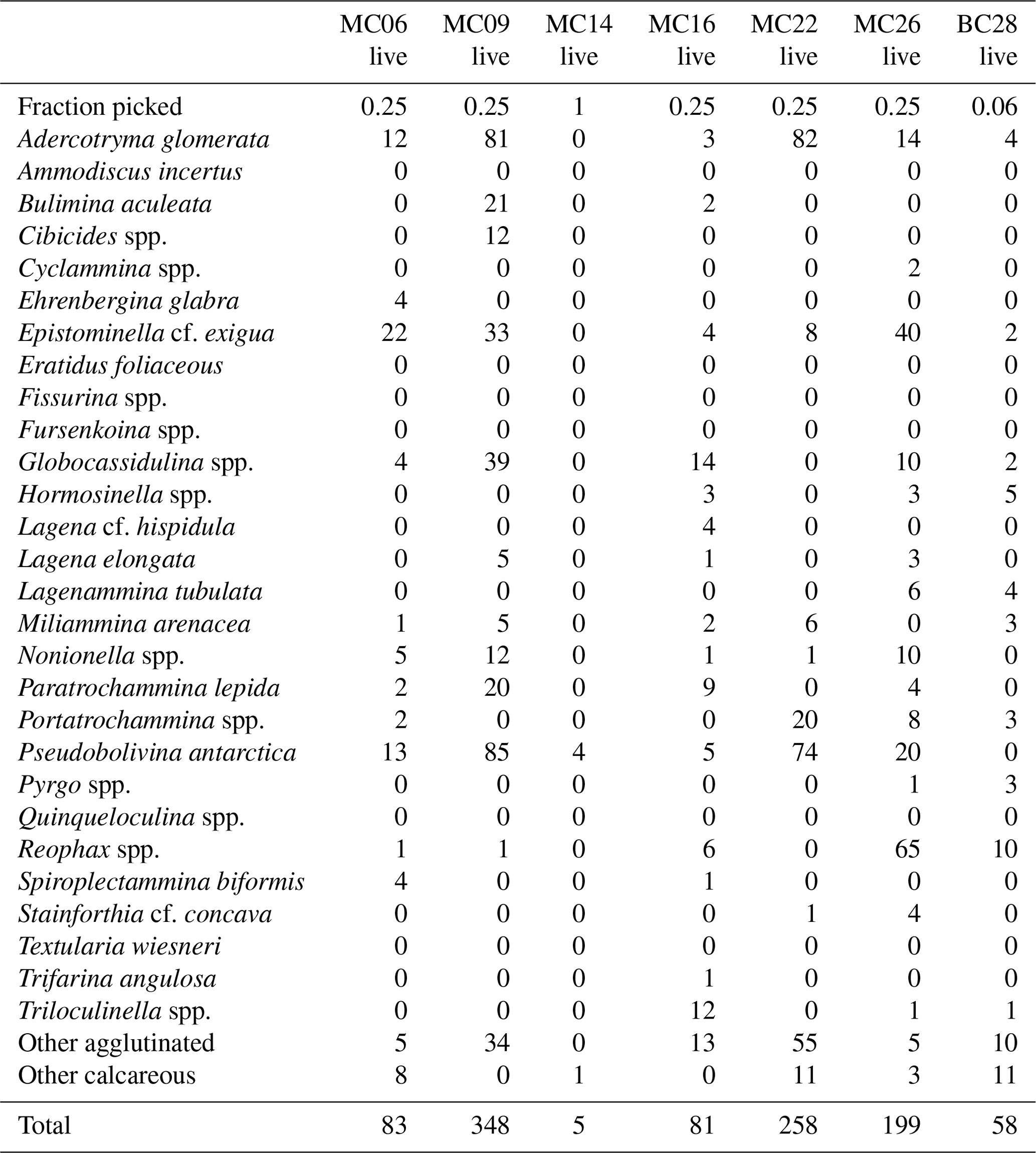
Table 3 Benthic foraminifera species numbers in live populations of NBP19-02 surface sediment samples. MC14 is not considered further in the statistical analyses due to low numbers of foraminifera tests.

2.3 Sample processing

Surface samples from the top 1 cm of core were immediately submerged in a 1 g L⁻¹ rose bengal/ethanol solution (Walton, 1952) in a 1 L Nalgene bottle. In total, 95 cc of sediment were stained from all cores, except MC06, which had limited surface material available, so only 65 cc were stained. Samples were gently agitated for a minimum of 24 h, in line with the minimum staining time applied in other studies (e.g., Bernhard et al., 2006), and a maximum of 3 d. We acknowledge that in the literature there is no consistency regarding the time applied for the staining of foraminifera samples with rose bengal, and minimum times of 24 h up to several weeks have been used or recommended (e.g., Bernhard et al., 2006; Schönfeld et al., 2012; Majewski et al., 2023). We used this (minimum) time protocol in accordance with environmental regulations aboard RV/IB Nathaniel B. Palmer with the relatively high proportion of stained foraminifera in the analyzed samples suggesting effectiveness (Tables 3, 4, 5). Discrepancies in protocols between studies may have implications for interpretations, and thus standardization in the field of living benthic foraminifera studies will be useful in the future (e.g., recommendations in Schönfeld et al., 2012).

Wet bulk sample weight could not be measured before sieving on board due to the sea state. Samples were sieved at 63 µm with tap water. A mesh size of 63 µm was chosen to maximize the retention of sand-sized foraminiferal tests, while also retaining small species and juvenile forms. Samples were placed in a gravity convection oven at 40 °C until dry and were stored in glass vials until they could be investigated under reflected light using a Swift Zoom Stereo microscope (1$\times -\mathrm{4}\times$ with 10× viewfinder). The sand samples were split using a micro-splitter to allow other proxies to be measured on foraminiferal tests from the other splits; thus, this study investigated a fraction of the initially stained sample (Tables 3, 4). All foraminiferal specimens were then dry-picked and separated based on staining from the split samples.

Table 4 Benthic foraminifera species numbers in dead assemblages of NBP19-02 surface sediment samples. MC14 is not considered further in the statistical analyses due to low numbers of foraminifera tests.

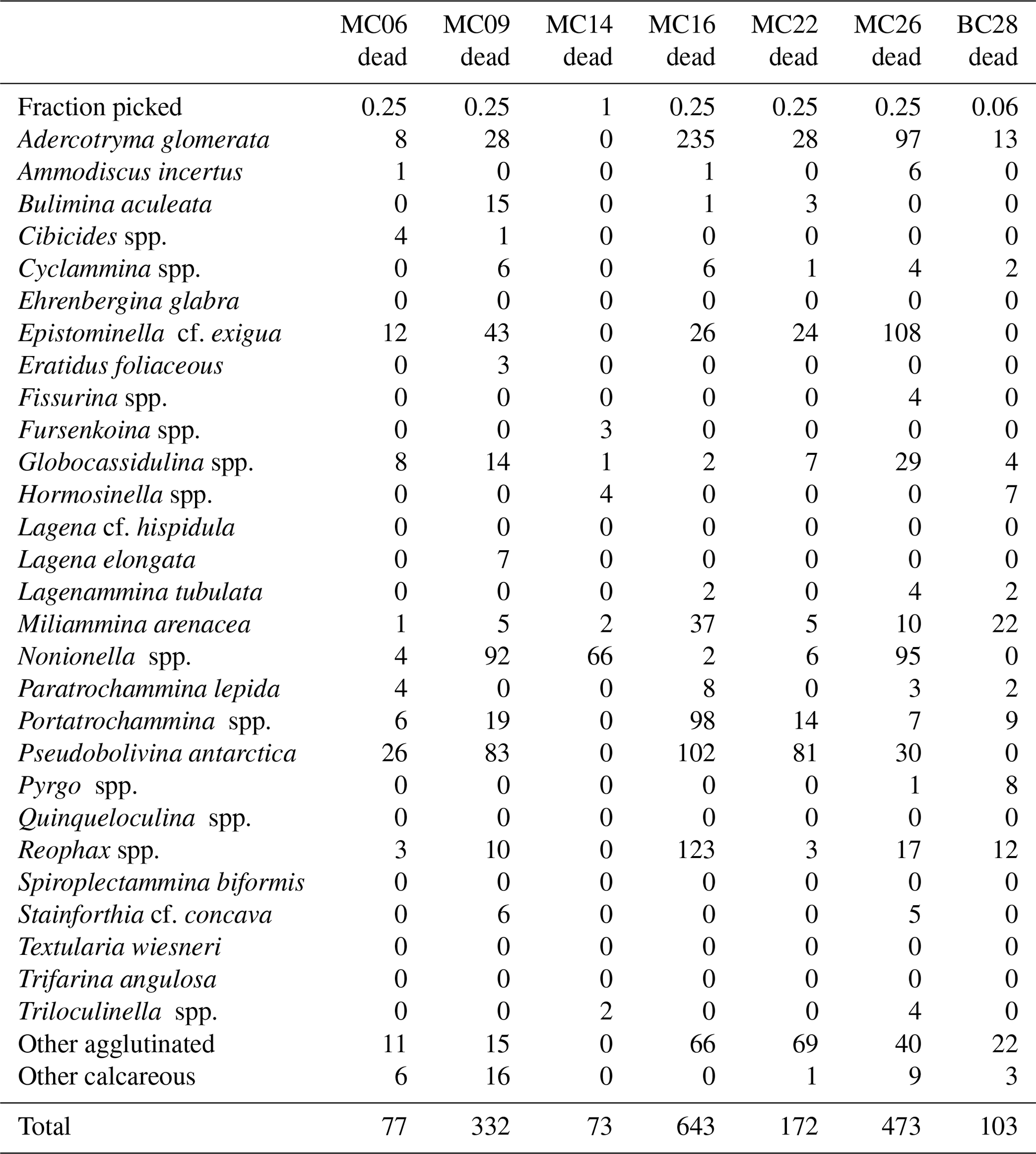
Table 5 Faunal parameters of live benthic foraminiferal assemblages in NBP19-02 surface sediment samples.

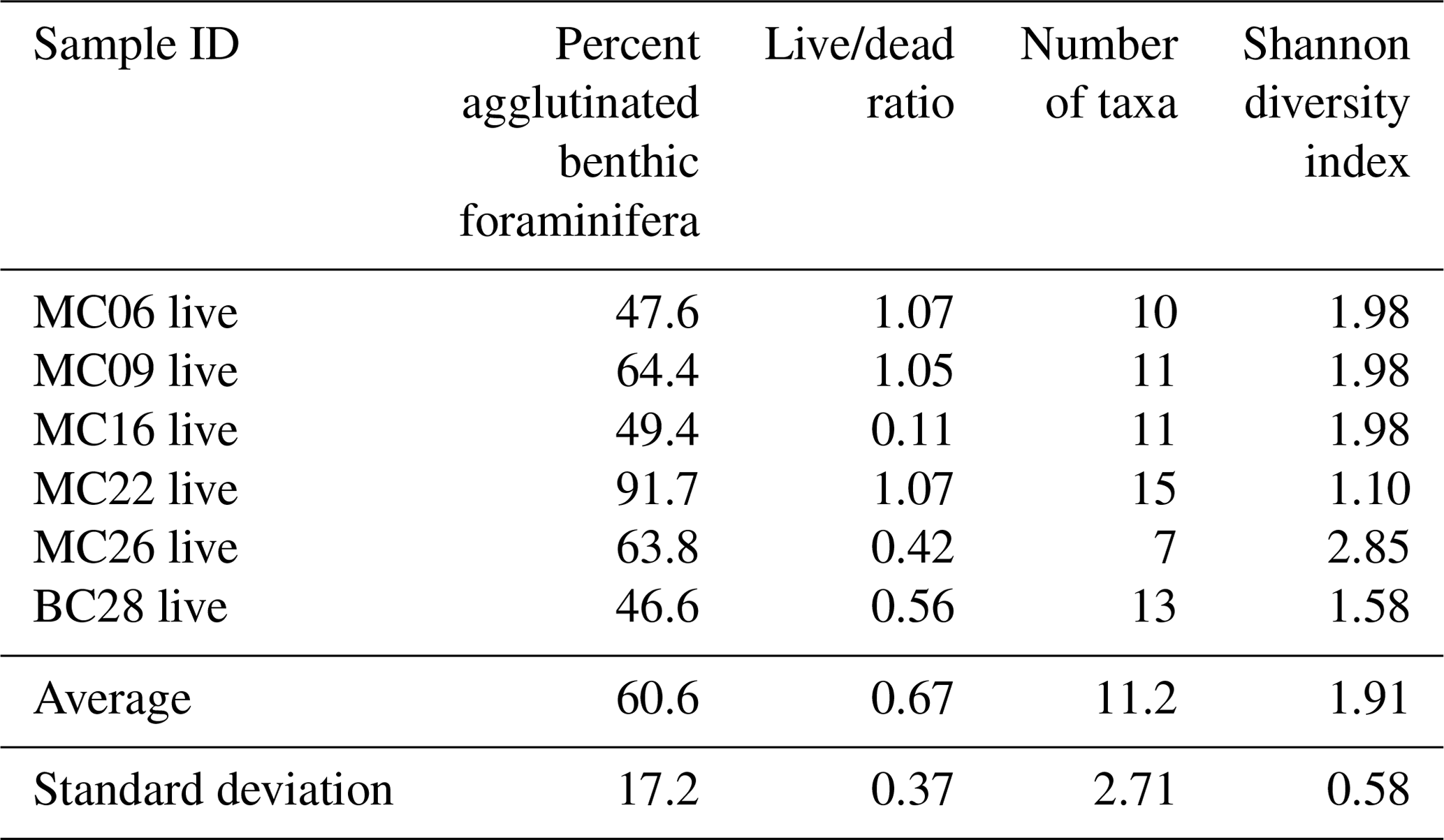
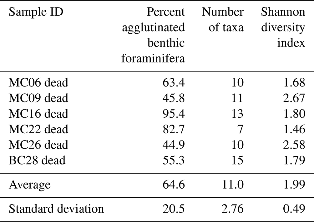
Table 6 Faunal parameters of dead benthic foraminiferal assemblages in NBP19-02 surface sediment samples.

The classification scheme chosen for the order Foraminiferida follows Loeblich and Tappan (1988), and the taxonomic identifications follow Majewski (2010, 2013), with accepted naming conventions from Hayward et al. (2024). It is recommended to count at least 300 specimens for statistical significance (i.e., Patterson and Fishbein, 1989). However, due to the small quantities of stained/unstained foraminifera present in some of the samples (Tables 3, 4), fewer than 300 were counted in the corresponding samples.

Benthic foraminiferal tests that were identified by the visible pink staining of rose bengal within tests were considered alive at the time of sample collection (Murray and Bowser, 2000). Unstained or partly stained specimens, where only the exterior of the test was stained, were considered dead at the time of collection because it is likely that only surface-adhering microbes were stained in the latter (Murray and Bowser, 2000).

To characterize the seafloor substrate, grain size analysis was conducted. A surface sediment sample of ∼ 5 cc volume was taken from an unstained sub-core for the grain size analysis. The sample was dispersed using tap water and a deflocculating agent, sodium hexametaphosphate, and allowed to sit for a minimum of 48 h. The sample was then homogenized with a magnetic stirrer, and a subsample was taken with a pipette for analysis. The grain size was measured using a Cilas 1190 laser particle size analyzer. The median (D50), percentiles (D10 and D90), and mean grain size were determined by the Cilas software.

Table 7 Benthic foraminifera percentages in live populations of NBP19-02 surface sediment samples.

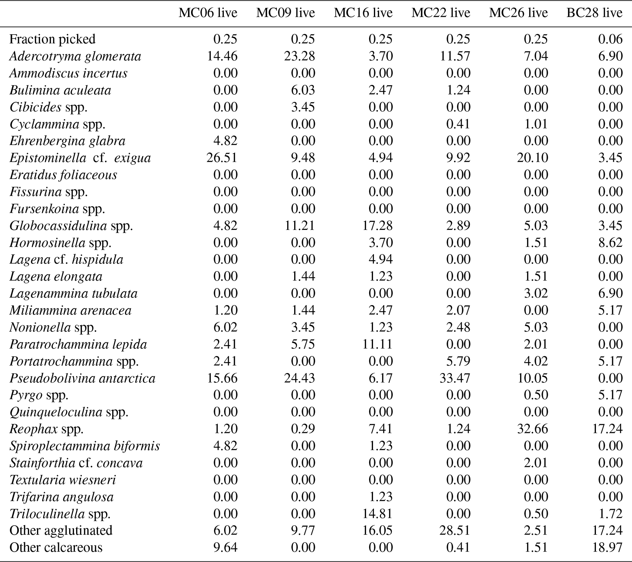
Table 8 Benthic foraminifera species percentages in dead assemblages of NBP19-02 surface sediment samples.

2.4 Dataset analyses

The benthic foraminiferal genus/species counts are presented as total numbers (Tables 5, 6) and percentages (Tables 7, 8), but only percentages were used for statistical analyses. This approach eliminates challenges associated with the interpretation of absolute data (Majewski et al., 2016).

To evaluate the faunal diversity of each sample, the Shannon diversity index was employed, $H=-\mathrm{\Sigma }{n}_i/n\ln (n_i/n)$, with n_i being the number of individual species (Shannon, 1948). As in other studies in which there is uncertainty in taxonomy (e.g., Majewski, 2013), taxonomic lumping to the genus level has been included in H, and there is a higher error in H with more taxonomic lumping (Wu, 1982). As we only compare H between sites in this study, and each site has the same identification scheme, we assume a constant error.

A correlation matrix between foraminiferal genus/species percentages and environmental parameters was used as input to the Python package pandas v2.2.2 with the function “corr()” to compute a linear relationship between each pair of variables (McKinney, 2010; Pandas Development Team, 2024). The graphic of this computation was created using the Python packages matplotlib v3.9.1 (Matplotlib Development Team, 2024) and seaborn (Waskom, 2021) and color schemes from cmcrameri v.8.0.0 (Crameri, 2023).

Table 9 Live assemblage principal component analysis (PCA) loadings by species, samples, eigenvalues, and percent variance. Significant principal components are shown in bold.

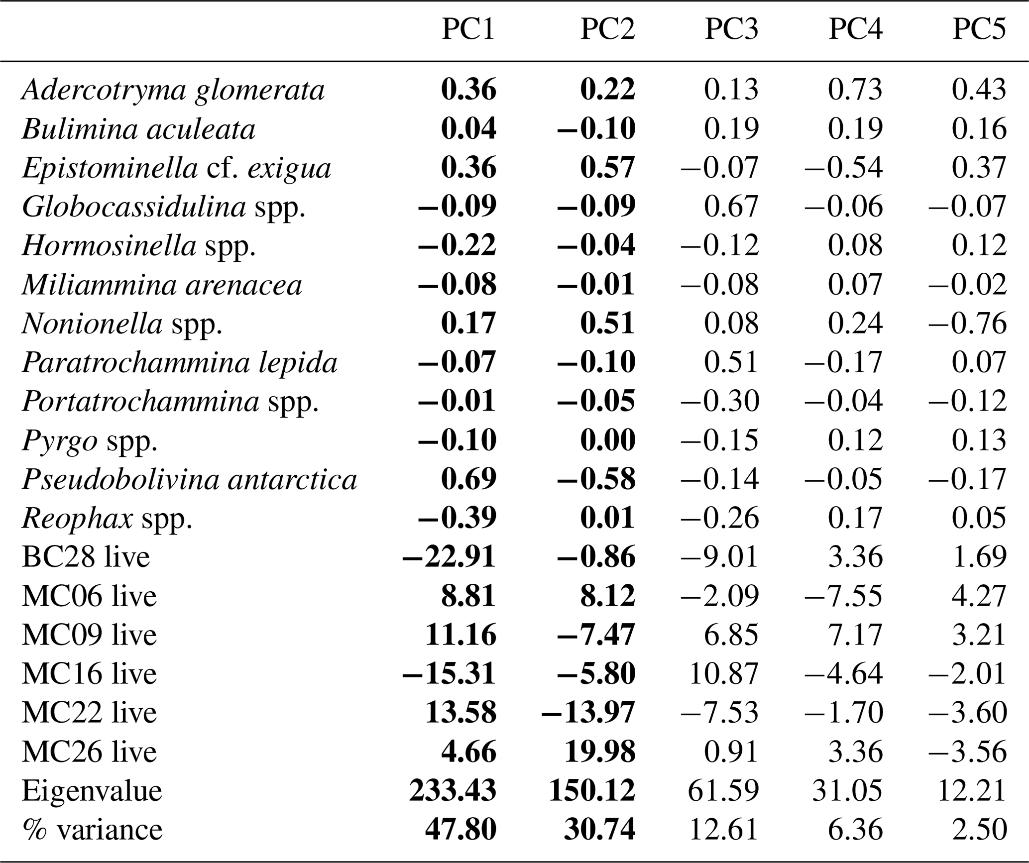
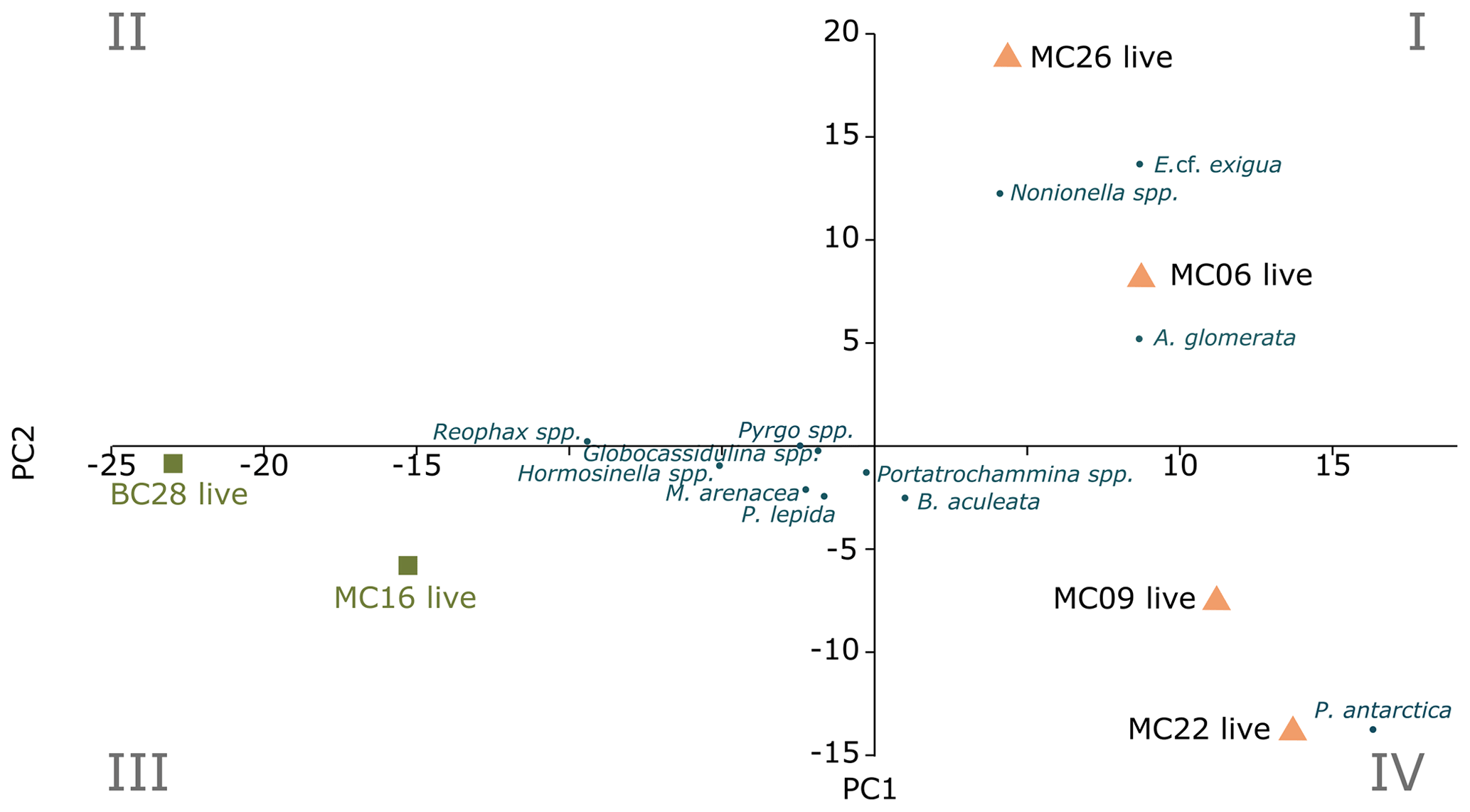
Figure 3 Foraminiferal populations (FPs) of live benthic species, with PC1 on the x axis and PC2 on the y axis. The blue dots are species inputs of the PCA. The Miliammina arenacea foraminiferal population (FP) lies in quadrant III, and the corresponding samples are marked by green squares. The Epistominella cf. exigua FP lies in quadrants I and IV, with the corresponding samples marked by orange triangles.

The R-mode principal component analysis (PCA) in PAST4 (Hammer et al., 2001) was applied to the live foraminiferal census percentages of six samples (described in Sect. 3.2), i.e., MC06, MC09, MC16, MC22, MC26, and BC28, to find hypothetical variants/components accounting for the variance in the data that comprise species taxonomic groups above a frequency of 3 % (Table 9; Fig. 3; Davis, 1986; Legendre and Legendre, 1998; Harper, 1999). A second R-mode PCA was applied to the total foraminiferal census above a frequency of 3 %, including the dead specimens (Table 10). PCA uses a single-value decomposition algorithm to find eigenvalues and eigenvectors, which identify the proportion of variance per component, and plot these components.

To determine which components are statistically significant, a Scree test (Figs. 4, 7) was employed by plotting components by eigenvalue (Cattell, 1966). The components that lie above the break, or “elbow”, of the plot are determined as significant. To aid in creating the grouping within the PCA, R-mode cluster analyses from PAST4 (Hammer et al., 2001) were used. Classical clustering with the unweighted pair group method with arithmetic mean (UPGMA) produces clusters based on the average distance between all members (Sokal and Michener, 1958). Each cluster has the same branch length as its internal node.

Table 10 Total assemblage PCA loadings by species, samples, eigenvalues, and percent variance. Significant principal components (PCs) are shown in bold.

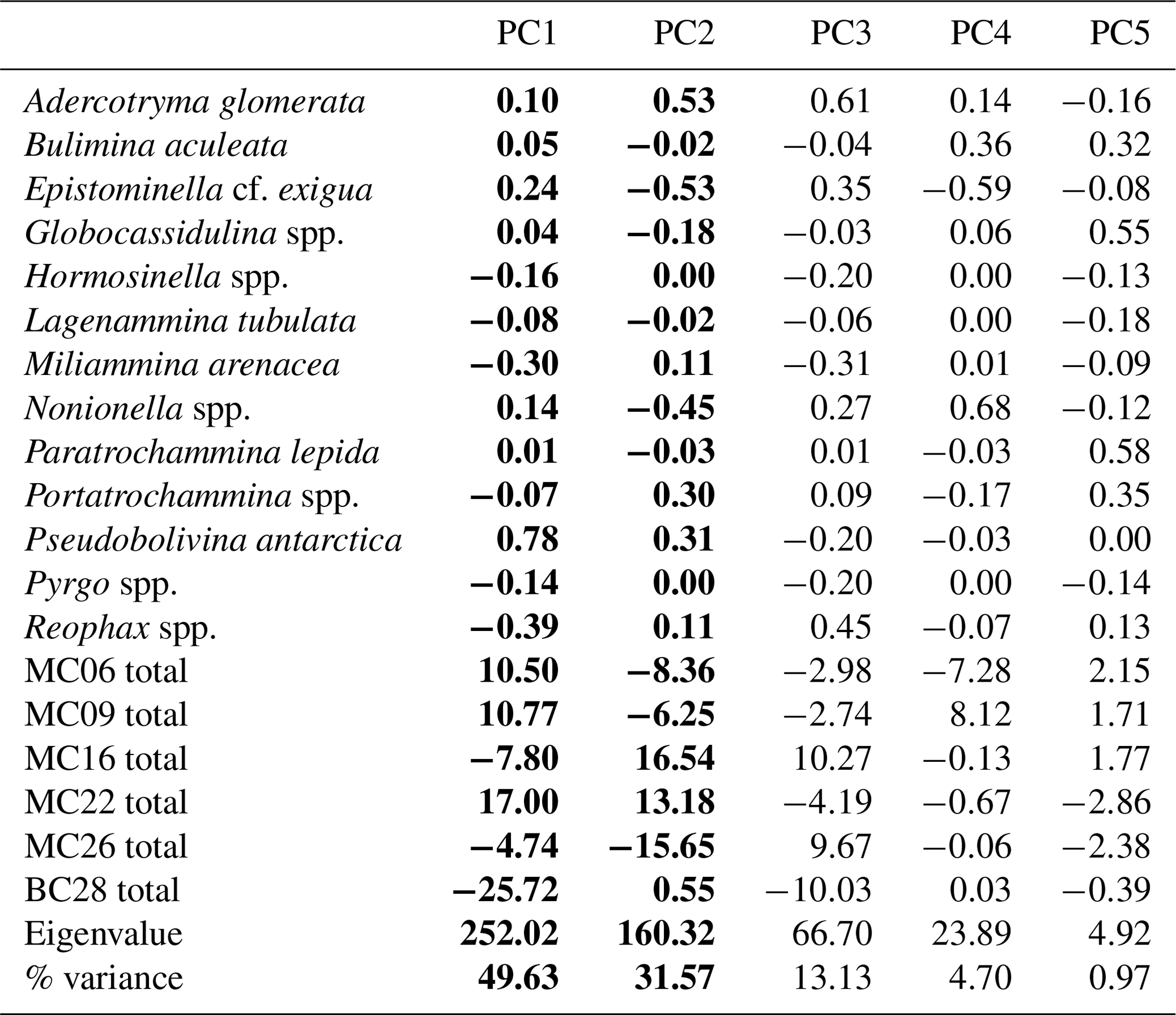
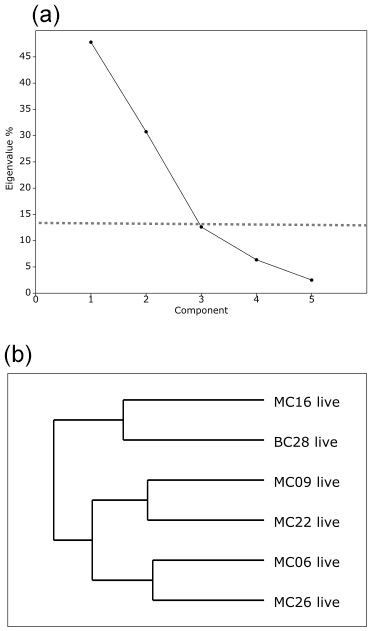
Figure 4 (a) Scree analysis of live population PCA from PAST4 to determine the statistically significant principal components (PCs) of the live assemblage. Components below the horizontal dashed line are not statistically significant. (b) Hierarchical cluster analysis aids in determining the groupings within the PCA.

3 Results

3.1 Bottom-water and substrate properties

At the deepest sites of this study, MC09 (1138 m water depth) and MC22 (1022 m water depth), relatively warm and saline bottom water was observed, with a temperature of 1.1 °C and a salinity of 34.7 PSU (Fig. 1b; Tables 1, 2). These conditions fall within the CDW properties documented near Thwaites Glacier in the same season (Wåhlin et al., 2021). Bottom water at site MC26 from 557 m water depth has a slightly lower temperature of 0.2 °C and a slightly lower salinity of 34.6 PSU, although these also match modified CDW properties (Fig. 1; Table 1). Sites MC06, from 467 m water depth, and MC16, from 549 m water depth, are characterized by cooler and fresher bottom water, with temperatures of −0.5 and 0.3 °C and lower salinities of 34.3 and 34.5 PSU, respectively (Fig. 1; Table 1). Each of these sites is located proximal to Thwaites Glacier, and the mean grain size of each sample ranges from 8 to 13 µm, i.e., fine silt (Folk, 1954), and 90 % of the material is finer than 24 µm (Table 2).

Site BC28 from 645 m water depth in Cranton Bay is characterized by relatively cold (−0.7 °C) and fresh (34.3 PSU) bottom water. In the data collected for this study, this is the only site not influenced by unmodified or even modified CDW, likely due to its location to the east of the main pathway of CDW flow through Pine Island Trough (Fig. 1; Table 1). The concentration of DO in the bottom water at the Cranton Bay site is higher than at all other sites, suggesting that the bottom water of Cranton Bay recently exchanged with the atmosphere (Table 1). Although also silt-dominated, the surface sediment at this location is coarser than at the sites proximal to Thwaites Glacier, with a mean grain size of 18 µm (i.e., medium silt) and 90 % of the sediment being finer than 42 µm (Table 2).

3.2 Benthic foraminiferal census

A total of 2905 benthic foraminiferal specimens, of which 1032 were “live” (rose-bengal-stained), were counted and identified from six of the seven samples (Tables 3, 4). Because the sample from site MC14 only contained 5 living foraminiferal specimens and 73 dead foraminifera, it was not investigated further in this study and is not considered further in the statistical analyses due to its low sample numbers.

Among the specimens counted, 29 taxonomic groups were recognized. If a species could not be reliably identified, specimens were grouped by genera. Species that are problematic to identify, such as Globocassidulina biora and G. subglobosa (Majewski and Pawlowski, 2010) and species belonging to the genus Portatrochammina (Majewski, 2013), were also grouped by genus. Unidentified specimens were categorized into the groups “other calcareous” or “other agglutinated”, depending on their test compositions. The taxonomic groupings are referred to as “species” from here onwards.

The most abundant species in the total population are Adercotryma glomerata, Pseudobolivina antarctica, Nonionella spp., and Epistominella cf. exigua (Tables 3, 4). The most abundant living species are the arenaceous A. glomerata and P. antarctica (Table 3). The most abundant taxa in the dead census are also A. glomerata and P. antarctica (Table 4). MC22 is the sample with the highest percentages of agglutinated specimens in the living population and MC16 in the dead assemblage (Tables 5, 6).

The numbers of living foraminifera in all samples, except MC09, are below the recommended standard of 300 specimens per sample, while (apart from MC14) only samples MC06 (smallest stained sample volume) and BC28 (smallest split) have fewer than 300 specimens in total, i.e., live plus dead, of foraminifera (Tables 3, 4). This shortfall has the potential to introduce bias into statistical analyses and interpretations. Nevertheless, in regions difficult to access and with limited calcite preservation, such as the Amundsen Sea, any available samples and data should be utilized. We refrain from dismissing the data from the investigated sites, while simultaneously exercising caution in their interpretation.

The benthic foraminiferal census is discussed from west to east across the study area. Located in Thwaites Trough (Figs. 1, 2), sample MC09 contained 680 foraminiferal specimens of which 348 were alive and 332 were dead (Tables 3, 4). Thus, 51 % of the benthic foraminifera were alive at the time of collection (Table 5). There were 11 species alive identified in this sample, and the agglutinated species P. antarctica and A. glomerata are most abundant in the living population (Table 7). P. antarctica is the most abundant species in the thanatocoenosis, along with Nonionella spp. (Table 8). Bulimia aculeata has its highest abundance in sample MC09, accounting for 6 % of the living population (Table 7).

Located directly offshore from TGT in a localized basin on top of a bathymetric high referred to as “H2” (Figs. 1, 2; Hogan et al., 2020), sample MC06 contained 160 foraminiferal specimens, of which 83 were alive and 77 were dead (Tables 3, 4). E. cf. exigua and P. antarctica are most abundant in the living and dead assemblages, with the former being the most abundant species in the biocoenosis and the latter being the most abundant species in the thanatocoenosis (Tables 7, 8). It should be noted that although the tests of E. cf. exigua have a thin wall, its hyaline composition is resistant to dissolution from carbonate corrosive waters (e.g., Anderson, 1975; Ishman and Szymcek, 2003).

Sample MC22 from bathymetric trough T3 (Figs. 1, 2) contained 430 foraminifera, of which 258 were alive and 172 were dead (Tables 3, 4). The live foraminifera accounted for 55 % of the total assemblage (Table 5). The most common species of both the live and dead assemblages are the agglutinated foraminifera A. glomerata and P. antarctica (Tables 7, 8).

Further north, on the SW flank of the “H1” bathymetric high (Hogan et al., 2020), sample MC16 contained 724 foraminifera, of which 81 specimens were alive and 643 were dead (Figs. 1, 2; Tables 3, 4). Only 11 % of the total assemblage was alive at the time of collection (Table 5). Globocassidulina spp. and Triloculinella spp. are the most abundant species in the live population (Table 7). A. glomerata (37 %) is the most abundant species in the dead assemblage (Table 8). Of all the studied samples, MC16 and MC09 are the only ones containing live B. aculeata (Table 3).

Between the EIS and Pine Island Glacier lies site MC26 (Fig. 1). The sample from this location contained 672 specimens, including 199 living specimens and 473 dead specimens (Tables 3, 4). The most abundant species are Reophax spp. and E. cf. exigua in the live population and E. cf. exigua and A. glomerata in the dead assemblage (Tables 7, 8). A. glomerata accounts for 21% of the dead population but only 7 % of the live population, while E. cf. exigua accounts for 20 % and 23 % of the live population and the dead assemblage, respectively (Tables 7, 8).

In sample BC28 from Cranton Bay (Fig. 1), which is characterized by less sea ice cover and coarser-grained substrate than the other samples, 161 foraminifera were found, of which 58 were alive and 103 were dead (Tables 3, 4). In the biocoenosis, Reophax spp. is the most abundant species, while M. arenacea and A. glomerata are the most abundant in the thanatocoenosis (Tables 7, 8). Notably, foraminiferal tests in this sample appeared visually larger than in all the other studied samples.

3.3 Benthic foraminiferal populations (FPs)

3.3.1 Live (stained) benthic FPs

Application of the Scree test (Cattell, 1966) to the live FP PCA demonstrates that the first two axes of variance, the principal components (PCs), are statistically significant (Fig. 4a). Of the living foraminifera variance, 78 % are represented in this model, with 48 % by PC1 and 31 % by PC2 (Fig. 3; Table 9). Because PC3 does not account for statistically significant variability, it is not described or discussed further.

Classical clustering revealed two clusters or FPs (Fig. 4b). One cluster contains MC16 and BC28. Within the PCA model, this cluster lies within quadrant III (Figs. 3, 4). This cluster is characterized by Reophax spp., Hormosinella spp., Globocassidulina spp., M. arenacea, Paratrochammina lepida, Pyrgo spp., and Portatrochammina spp. (Fig. 3). Reophax spp., M. arenacea, and Pyrgo spp. are negatively correlated with bottom-water temperature, salinity, and sea ice presence and positively correlated with DO (Fig. 5). Globocassidulina spp. is positively correlated with temperature and negatively correlated with DO (Fig. 5).

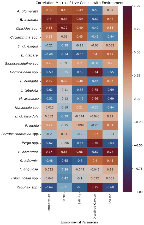
Figure 5 Correlation matrix of living foraminiferal species/genera and environmental parameters. Warmer/red colors indicate a positive correlation, and cooler/blue colors indicate a negative correlation.

The second cluster contains MC06, MC09, MC22, and MC26, all of which are plotted along the positive PC1 axis (Figs. 3, 4b). The subcluster containing MC06 and MC26 lies in quadrant I and is characterized by E. cf. exigua, Nonionella spp., and A. glomerata (Fig. 3). E. cf. exigua is negatively correlated with water depth; however, A. glomerata is positively correlated with water depth (Fig. 5). It should be noted that E. cf. exigua does not have strong correlations with other environmental parameters (Fig. 5). A. glomerata is positively correlated with water temperature and salinity and negatively correlated with DO and sea ice coverage, which is a proxy for restriction in nutrient/food supply (Fig. 5). Nonionella spp. is negatively correlated with sea ice cover.

The other subcluster lies in quadrant IV with MC09 and MC22 and is characterized by P. antarctica, Globocassidulina spp., and B. aculeata (Figs. 3, 4b). P. antarctica and B. aculeata are positively correlated with water temperature, salinity, water depth, and sea ice (Fig. 5). P. antarctica and B. aculeata are negatively correlated with DO (Fig. 5). Globocassidulina spp. is positively correlated with temperature and negatively correlated with DO (Fig. 5).

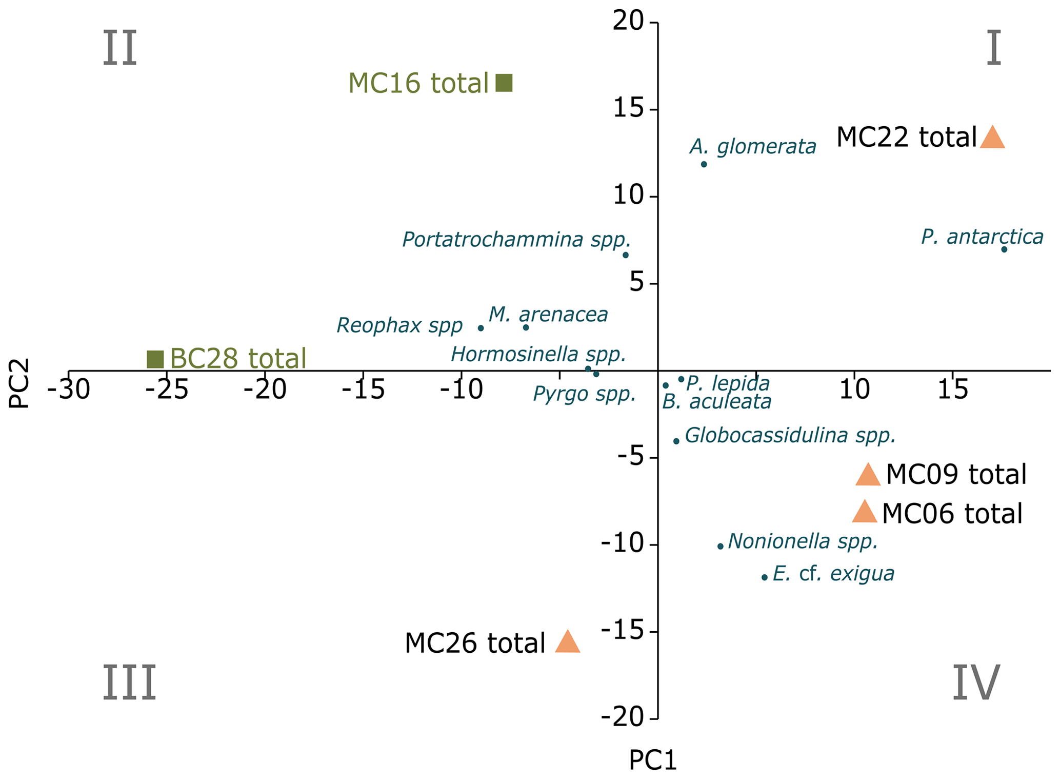
Figure 6 Foraminiferal assemblages (FAs) of living and dead foraminifera, with PC1 on the x axis and PC2 on the y axis. The blue dots are species inputs of the PCA. Portatrochammina spp. FA lies in quadrant II, and the corresponding samples are marked by green squares. E. cf. exigua FA lies in I and IV, and the corresponding samples are marked by orange triangles.

3.3.2 Total (live and dead combined) foraminiferal assemblages (FAs)

In the total foraminifera PCA, the Scree test (Cattell, 1996) determined that only the first two PCs are statistically significant (Figs. 6, 7a; Table 10). Of the total foraminifera variance, 50 % is on PC1, and 32 % is on PC2, accounting for 82 % of the total variance (Figs. 6, 7a, 10b). Classical clustering revealed two clusters (FPs), including samples BC28 and MC16 in quadrant II, sample MC22 in quadrant I, MC26 in quadrant III, and MC06 and MC09 in quadrant IV, respectively (Figs. 6, 7b). This division of the core samples into different clusters is the same as described above for the live FPs.

The cluster in quadrant II is characterized by the agglutinated foraminifera M. arenacea, Portatrochammina spp., and Reophax spp. (Fig. 6; Table 10). Portatrochammina spp. is negatively correlated with water temperature (Fig. 8). Reophax spp. is strongly negatively correlated with sea ice cover, water temperature, and water depth (Fig. 8). M. arenacea is strongly positively correlated with DO and negatively correlated with sea ice cover and water temperature (Fig. 8). Thus, the unifying qualities of this FP are cooler water temperature and relatively more open-water conditions.

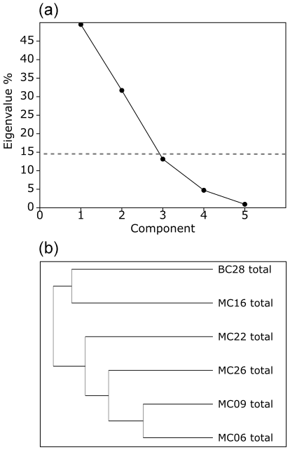
Figure 7 (a) Scree analysis of total assemblage PCA from PAST4 to determine the total live and dead assemblage statistically significant components (PCs). Components below the horizontal dashed line are not statistically significant. (b) Hierarchical cluster analysis aids in determining the groupings within the PCA.

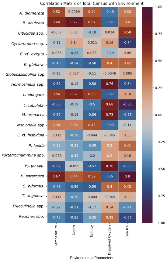
Figure 8 Correlation matrix of total census of foraminiferal species/genera and environmental parameters. Warmer/red colors indicate a positive correlation, and cooler/blue colors indicate a negative correlation.

The second cluster in the thanatocoenosis is not divided into subclusters, unlike that for the live FPs. The second cluster is distributed across quadrants I, III, and IV, and it is characterized by E. cf. exigua, P. antarctica, Nonionella spp., A. glomerata, Globocassidulina spp., B. aculeata, and P. lepida (Figs. 6, 7b). E. cf. exigua, though most statistically significant and abundant in this cluster, is weakly correlated with the environmental parameters, including temperature, salinity, DO, and sea ice conditions (Fig. 8). Like E. cf. exigua, A. glomerata and Globocassidulina spp. are only weakly correlated with the environmental parameters. As in the live population, P. antarctica and B. aculeata are strongly positively correlated with sea ice coverage and water temperature, salinity, and water depth and strongly negatively correlated with DO (Fig. 8). Nonionella spp. is positively correlated with water temperature (Fig. 8). Thus, the unifying characteristics of this cluster are water temperature, salinity, and water depth, and relatively more sea ice coverage.

The hydrographic parameters included in this study are derived from CTD casts, which represent only a snapshot of the environmental conditions during the period of the accumulated total foraminiferal assemblage. Even with this limitation, the evaluation of each species' ecologic affinity is valuable because this is the only study in the Amundsen Sea region that compares in situ environmental data with live foraminiferal populations.

4 Discussion

4.1 Differences between live and dead benthic foraminiferal assemblages in ice proximal samples

The dead benthic foraminiferal census preserved in seabed sediments usually varies from the live census (Murray, 1982; Murray and Alve, 2011). Preservation bias, often as a result of post-mortal dissolution of calcareous foraminifera, or preferential loss of weakly cemented agglutinated foraminifera can cause this difference. Along with preservation bias, there is an inherent difference between the live and dead census because the dead census represents many generations of foraminifera, with the number of generations depending on multiple elements, including the sedimentation rate. Furthermore, the changes in population in response to seasonality or other changing environmental conditions can also cause variance between the live and dead census (Murray, 1982). Therefore, it cannot be assumed that the “snapshot” of the environmental conditions, as recorded from the CTD data during the collection of our samples, is representative of the environmental conditions prevailing during the period over which the total assemblage accumulated. Furthermore, it is impossible to know exactly how many specimens were lost due to preservation bias.

At sites MC09 and MC22, the live/dead ratios are high, implying that the total assemblage is similar to the live population (e.g., Murray, 1982). However, close inspection of the dominant foraminiferal species in sample MC09 reveals biases in the thanatocoenosis. For example, while the percentages of B. aculeata in the live and dead assemblages are nearly the same (6 % and 5 %, respectively), the agglutinated species A. glomerata accounts for 23 % of the live population but only 8 % of the dead assemblage (Tables 7, 8). Conversely, at site MC22, a lower abundance of A. glomerata in the biocoenosis (12 %) compared to the thanatocoenosis (16 %) is observed. Both MC22 and MC09 are located in deep troughs below 1000 m water depth (Fig. 1). At such deep-water locations, some agglutinated foraminiferal species can have a reduced preservation potential in the dead assemblage (e.g., Balestra et al., 2017) as we observe for A. glomerata in MC09. This is believed to be due to the increased decay of species with weakly cemented agglutinated tests via the microbial respiration in deeper water (e.g., Murray and Pudsey, 2004). However, this scenario is not supported by our results regarding the post-mortem preservation of A. glomerata from site MC22.

There are other possible reasons for the differences in the living populations and the dead assemblages. The aforementioned differences between live and dead assemblages in sample MC09 perhaps result from the calving of the large iceberg B22 from Thwaites Glacier's ice shelf in 2002 CE, its subsequent temporary grounding just to the northwest of the site, and the mélange of sea ice and smaller icebergs that had formed between TGT and B22 after its grounding until the mélange broke up before the samples were collected in 2019 CE (e.g., Stammerjohn et al., 2015; Miles et al., 2020). This could have contributed to a shift in environmental conditions, i.e., the dead assemblage may predominantly represent a sub-ice melange setting, whereas the live population may mainly reflect the more recent ice-proximal and seasonally open-water conditions after the mélange break-up (Fig. 1). However, without continuous oceanographic and ecological observational data collected from this location during the time represented by the sample, it is difficult to test this hypothesis. Surficial sedimentation rates across the Thwaites study area, derived from ²¹⁰Pb chronologies, range from ∼ 4 mm yr⁻¹ at site MC16 between the EIS and TGT to ∼ 2 mm yr⁻¹ at site MC06, which was recovered from the same site as KC04 on a bank just offshore of the TGT (Clark et al., 2024). Our surface samples are taken from the top 1 cm of the cores and, therefore, probably represent between 2.5 and 5 years of time, depending on the location.

One hypothesized indicator for CDW, B. aculeata (Ishman and Domack, 1994; Majewski, 2013), is only present in the live and dead census of MC09 and MC16 and in the dead census of MC22 (Tables 7, 8). The similar proportions of B. aculeata in the live and dead assemblages of sample MC09 may be related to the CDW inflow assumed to affect this site (Wåhlin et al., 2021). However, in trough T3, where CDW has also been documented during the time of sample collection (Wåhlin et al., 2021), B. aculeata is absent in the live MC22 census. Unlike sites MC09 and MC22, site MC16 was collected from a shallower setting at 549 m water depth (Fig. 1a) and is influenced by the longest open-water conditions of the sample localities most proximal to the Thwaites Glacier front (summer sea ice cover was 78 %; see Table 1). Though our CTD data indicate a relatively cool water temperature of 0.3 °C, other studies clearly illustrate that MC16 lies on the CDW pathway (Wåhlin et al., 2021). We suggest that MC16 is situated in the uppermost part of the CDW layer, where mixing with cold surface and glacial meltwaters originating from the ice shelf front occurs. With CTD data agreeing that MC22 lies in one of the CDW flow paths (Wåhlin et al., 2021), a question arises with respect to why B. aculeata is absent from the living census of MC22.

Notably, sample MC16 contains the lowest proportion of live specimens in the total assemblage (only 11 %). Because this site is characterized by a higher sedimentation rate than that at our other sites, accumulation rates cannot be cited for the low proportion of live foraminifera. Environmental explanations for so few foraminifera surviving relative to the dead accumulation, including mass mortality due to changing oceanographic conditions, could be the cause of the low proportion of live foraminifera.

4.2 Dissolution influence on the preservation of calcareous species

Sample MC09 was collected from a water depth of 1138 m in Thwaites Trough to the west of the TGT (Fig. 1a) from below the local CCD on the Amundsen Sea shelf, which is assumed to lie at 300–500 m water depth (Kellogg and Kellogg, 1987) and ∼ 700 m water depth, respectively (Majewski, 2013). The presence of calcareous foraminifera at site MC09 was, therefore, unexpected. The abundance of calcareous specimens is comparable to that of agglutinated foraminifera, accounting for 36 % of the live population and even 54 % of the dead assemblage (Tables 5, 6). Calcareous foraminifera abundance at this deep site could indicate significant regional variations in the depth of the CCD throughout the Amundsen Sea Embayment, which apparently can lie deeper locally than previous foraminifera studies concluded, though selection of coring targets can introduce bias in the depth estimate for the CCD (Kellogg and Kellogg, 1987; Majewski, 2013).

Further confirming that the CCD can lie at greater water depth directly offshore from Thwaites Glacier, sample MC22 from 1022 m water depth in bathymetric trough T3 (Fig. 1a) still contains 8 % calcareous foraminifera in the live population (which is the lowest percentage of all live populations) and 17 % in the dead assemblage (Tables 5, 6). At site MC09 and site MC22 bottom-water properties and sea ice conditions are similar; temperature is 1.1 °C; salinity is 34.6 PSU; DO concentration is around 4.4 mL L⁻¹; and summer sea ice cover is 93 % and 90 %, respectively (Table 1). These conditions, especially the warmer bottom water, may allow a deeper CCD at sites MC09 and MC22 than elsewhere on the Amundsen Sea shelf, i.e., deeper than at the sites investigated by Kellogg and Kellogg (1987) and Majewski (2013).

For sediment sampling on expedition NBP19-02 in early 2019 CE, sites at water depths shallower than 700 m were preferentially targeted to increase the likelihood of calcite preservation in the sediment cores. At sites between 450 and 650 m water depth (sites MC06, MC16, MC26, and BC28), the proportions of calcareous foraminifera range from 5 % to 55 % in both the live and dead assemblages (Tables 5, 6) and thus illustrate that the water depth is not the only factor that should be considered for sampling carbonate-bearing sediments on the Amundsen Sea shelf (cf. Hauck et al., 2012). Nevertheless, our study illustrates that cores containing calcareous foraminifera can be retrieved from bathymetric troughs routing CDW directly offshore from Thwaites Glacier, even though it needs to be kept in mind that at sites MC09 and MC22, the proportions of calcareous benthic foraminifera in the live assemblages are the lowest of all studied samples (Table 5).

4.3 Diversity

Generally, the samples with relatively high diversity in the live population (MC22 and BC28) also show relatively high diversity in the dead assemblages (Tables 5, 6). In samples with low-diversity live populations (MC09 and MC26), there is also low diversity in the dead assemblages (Tables 5, 6). Apart from sample MC06, the diversity of each assemblage seems to be negatively correlated with water temperature (Tables 1, 5, 6). While we cannot compare the absolute abundances of foraminifera as the exact volumes of dry sediment of the sample splits are unknown, we can speculate that the deeper sites with warm-water influence (such as MC09 and MC22) host a community with lower diversity based on our counts. With that said, we acknowledge that in small sample sizes such as ours, rare species can be missed, thus biasing the results of species diversity.

4.4 Potential pioneer population

Directly offshore Thwaites Glacier, the bottom-water properties at site MC06 are different from its neighboring core sites, which creates a different habitat for the benthic fauna. This unique habitat offshore Thwaites Glacier causes a difference in the foraminiferal census, as exhibited by the differing foraminiferal species abundances and diversity (Tables 1, 5, 6, 8, 9). In the living census of MC06, the species E. cf. exigua prevails. However, in the dead census, E. cf. exigua abundance is closer in proportion to that of A. glomerata and Globocassidulina spp., while P. antarctica prevails (Tables 7, 8), indicating a preservation bias or a change in environment. The differences between the live and dead census in E. cf. exigua and agglutinated foraminifera may not be caused by calcite dissolution alone.

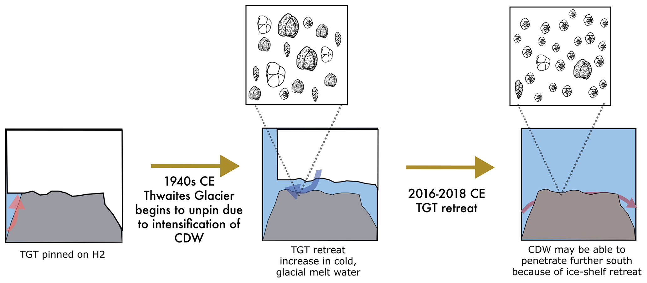
Figure 9 A pioneer population formed at H2 following ice retreat. TGT was pinned on H2 prior to the 1940s CE. TGT lifted off the seafloor from H2, beginning in the early 1940s (Clark et al., 2024), allowing for the foraminiferal community to adapt to cool water to establish. Cartoons of Adercotryma glomerata, Globocassidulina spp., E. cf. exigua, and Pseudobolivina antarctica generally represent the dead assemblage observed in the seafloor surface sample from site MC06. Ongoing ice shelf retreat, incursion of CDW, and establishment of the E. cf. exigua-dominated pioneer foraminiferal assemblage on H2 in seasonally open water. Cartoon shows E. cf. exigua dominating the foraminiferal assemblage at the site.

The observed changes in diversity and dominant foraminiferal species between the living and dead census may be significant. We propose that sample MC06 captured a faunal shift from environmental conditions, prevailing when the dead assemblage was alive, to the conditions recorded during the time the live population formed (Fig. 9). The sedimentation rate for the non-bioturbated seafloor surface sediments at site NBP19-02 KC04, retrieved from the same site as MC06, is 2 mm yr⁻¹ (Clark et al., 2024), implying that this assemblage shift must have occurred after 2013 CE and may reflect seafloor colonization by a pioneer foraminiferal community (Fig. 9). We note that E. cf. exigua, which prevails in the living population at site MC06, has been previously suggested to be an opportunistic species, which was able to thrive in food-limited environments with seasonal pulses of food, and has been associated with (seasonal) open-water and polynya conditions (e.g., Gooday and Rathburn, 1999; Ishman and Szymcek, 2003; Majewski et al., 2016). Core site MC06 was located close to the ice shelf front in 2019 CE (Fig. 1; Larter et al., 2020). Given the ice shelf edge retreat observed in this area over the last decade (Miles et al., 2020), we propose that the dead assemblage at site MC06 represents a sub-ice shelf assemblage influenced by cold and fresh meltwater from sub-ice-shelf melting, whereas the live population of MC06 has developed in response to the onset of seasonal open-water conditions following recent ice shelf front retreat.

We suggest that the live benthic foraminifera at site MC06 represent an evolving pioneer population in which the robust and generalist species E. cf. exigua could survive and thrive due to the rapid environmental changes affecting this location since ca. 2013 CE (Fig. 9; Milillo et al., 2019; Miles et al., 2020; Clark et al., 2024). Our FP and FA models (in Sect. 4.5 and 4.6 below) also indicate that the unique foraminiferal census of MC06 represents a pioneering population of a habitat in transition.

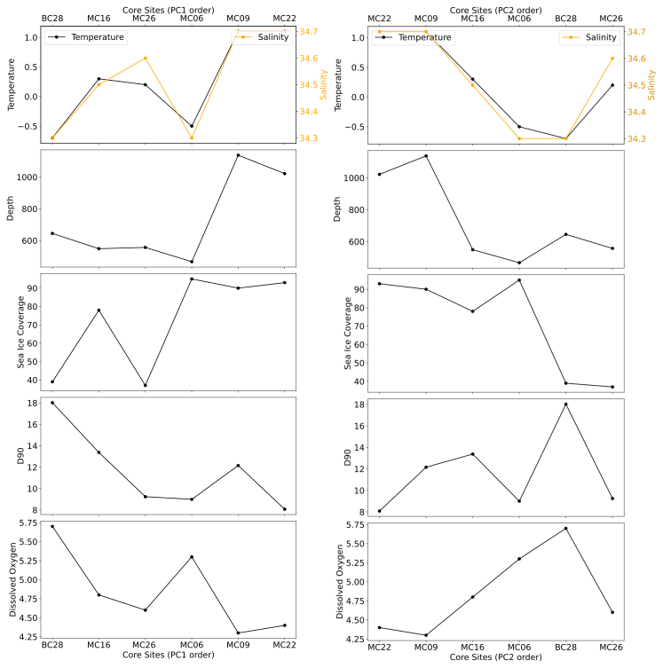
Figure 10 Living benthic foraminiferal assemblages at the studied sites, ordered according to PC1 (left panels) and PC2 (right panels), respectively, and plotted versus environmental parameters.

4.5 Live foraminiferal population (FP)

As the living FP model includes foraminifera counts with fewer than the standard 300 specimens per sample, there are inherent limitations. Despite this, we offer interpretations but simultaneously point out that the data basis needs to be improved in the future.

In the FP PCA models, there is a positive temperature gradient on PC1, except for the proposed pioneer assemblage of sample MC06, thus confirming our hypothesis that the water mass condition of temperature exerts a strong control on the FPs (Fig. 10). There is also a relationship of PC1 with water depth, which illustrates how deep channels acting as conduits for CDW (Hogan et al., 2020) influence the FPs.

Another control on the variance of the FP model is DO, which indicates the influence of meltwater (or exchange with the atmosphere) on deep-water properties. For the samples directly offshore TGT and EIS (except for site MC16), DO concentrations reflect the influence of meltwater along PC2. In MC09 and MC22, the relatively low DO indicates the presence of unmodified CDW. Both MC09 and MC22 are at the bottom of troughs, Thwaites Trough and T3, respectively, and the low DO could result from minimal meltwater contribution to CDW (see Wåhlin et al., 2021). MC06 from the H2 high (Fig. 1), from which TGT finally unpinned completely in 2011 CE (Rignot et al., 2014), has the highest DO concentration, indicating relatively high glacial meltwater influence. While the number of living benthic foraminifera in this sample is very low, we suggest that the variability observed in the live foraminiferal population is strongly related to the complex hydrography directly offshore of a rapidly retreating glacier–ice shelf system (Fig. 10).

The environment in and around Cranton Bay is characterized by oceanographic and glacial dynamics different from those at the other sample localities because no large glaciers drain into the bay and ice shelves are absent. Oceanographic information about Cranton Bay is limited. There were no direct interactions between CDW and cold glacial-melt-enriched water observed in Cranton Bay in the 2019 CE field season. It is likely that the high DO concentration, low temperature, and relatively low salinity in the bottom water at site BC28 (Table 1) originate from atmosphere–ocean interactions at the sea surface and/or sea ice melt.

PC2 is mostly controlled by summer sea ice cover, which controls phytoplankton production and hence food supply for the benthic fauna in the study area (Fig. 10). Sample locations with average summer sea ice cover (between 37 %–78 %) have more positive PC2 scores and localities with over 89 % summer sea ice cover have more negative PC2 scores (Fig. 10), which may indicate a relationship between foraminiferal species diversity and summer sea ice cover (Figs. 4, 5). This relationship excludes the proposed pioneer population of MC06.

Even though there are statistical limitations with the low number of living specimens in some of the samples, the FP model, using PCA in conjunction with classical cluster analysis, shows two clusters representing two distinct populations that are mostly defined by the environmental parameters characterizing PC1, namely temperature, salinity, and DO content of bottom water, as well as water depth (Figs. 4, 5). PC2 further defines these groups by summer sea ice cover (Figs. 4, 5).

4.6 E. cf. exigua FP

The first live FP cluster comprises samples MC06, MC09, MC22, and MC26 and the second cluster samples MC16 and BC28 (Fig. 3). The clusters are based on PC1 values, indicating the primary control of variance is water temperature, except for pioneer population MC06 (Fig. 3). The secondary control in this model is the presence of sea ice, as exhibited by PC2 (Table 1; Figs. 3, 5), which implies that the availability of a phytoplankton food source is the secondary environmental parameter. The first cluster is based on warmer bottom waters, and subclusters further categorize warm-water environments with phytoplankton food availability (except for the pioneer population in sample MC06). The cluster is characterized by E. cf. exigua, accounting for over 9 % of the live population, and generally a higher proportion of P. antarctica. Therefore, we refer to this FP as the E. cf. exigua FP. It is important to note that B. aculeata has a high statistical significance within the E. cf. exigua FP, although it is not an accessory species. As mentioned in Sect. 4.1, B. aculeata, previously established as a CDW indicator along the Antarctic Peninsula and in Pine Island Trough (Ishman and Domack, 1996; Majewski, 2013), is only present in MC09, MC16, and MC22. B. aculeata is most statistically significant in quadrant IV with MC09 and MC22, defining a subcluster of the E. cf. exigua FP (Fig. 4b). Because PC1 is controlled by water mass parameters, and because these two localities are the only ones in this dataset with relatively “pure” CDW properties, it can be inferred that quadrant IV indicates the presence of “pure” CDW. Thus, our results, although based on just six sampling sites, may suggest that only foraminifera communities from CDW-bathed locations with minimal glacial meltwater modification contain B. aculeata.

The other subcluster, MC06 and MC26 of quadrant I, is likely related to nutrient availability and relatively more glacially mixed CDW. This subcluster has the highest presence of E. cf. exigua in the study (Tables 7, 8). The pioneer population hypothesis (Sect. 4.4) posits that E. cf. exigua reflects seasonal nutrient availability. Furthermore, with seasonal open-water conditions at site MC26, E. cf. exigua has the opportunity to take advantage of increased phytoplankton flux. The low bottom-water temperatures at sites MC06 and MC26, −0.5 and 0.2 °C, respectively, indicate some glacial meltwater mixing with CDW (Table 1).

4.7 Miliammina arenacea FP

Within quadrant III of the FA model lies the cluster containing samples MC16 and BC28, with the unifying environmental parameters being low sea ice cover (i.e., more open-water conditions; Fig. 5; Table 1). With less than 78 % sea ice cover during austral summer, phytoplankton production at these sites can be expected to be higher than at the localities proximal to Thwaites Glacier's ice shelf front, especially TGT (Fig. 10; Table 1). Seafloor surface sediments from sample BC28 contained abundant siliceous microfossils including diatoms, confirming the hypothesis that there was significant phytoplankton production in Cranton Bay. The low sea ice cover at sites MC16 and BC28 is likely caused by PIP's northward extension into Cranton Bay (Stammerjohn et al., 2015; Herbert et al., 2023).

The calcareous benthic foraminiferal tests in sample BC28 tend to be larger and have thicker tests than those at the other sites (e.g., large Pyrgo spp. was observed at this site). The presence of Pyrgo spp. might be related to the high DO content in the Cranton Bay bottom waters, as this species is often associated with cold well-oxygenated waters (De and Gupta, 2010). Similarly, the agglutinated foraminifera of sample BC28 included visibly larger tests than the specimens at the other studied locations. Large calcareous and agglutinated benthic foraminifera thrive in Cranton Bay, suggesting that they live in a habitat with a more consistent and stable food supply in the austral summer compared to areas with more sea ice cover, which supports the hypothesis that PIP is the primary control of the FP.

The species with the most statistical significance of this FP are M. arenacea and Reophax spp., and the accessory species are Pyrgo spp., Hormosinella spp., and P. lepida. The agglutinated species Reophax spp. is problematic for downcore analyses because it does not preserve well below a seabed depth of >7 cm (e.g., Mackensen and Douglas, 1989; Murray and Pudsey, 2004). Because one of the objectives of this study is to refine the proxy for downcore analysis, and Reophax spp. is a problematic paleoenvironment proxy, we have named this assemblage the M. arenacea FP.

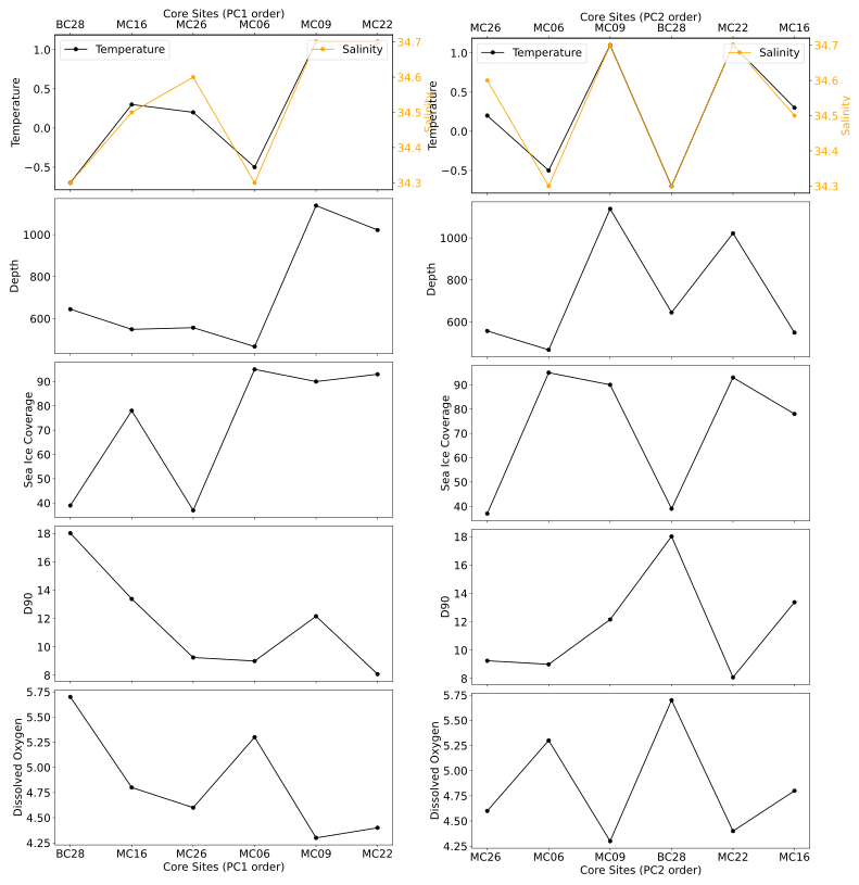
Figure 11 Total (i.e., living and dead) benthic foraminiferal assemblages at the studied sites, ordered according to PC1 (left panels) and PC2 (right panels), respectively, and plotted versus environmental parameters.

We do not exclude the possibility that the M. arenacea FP is geographically restricted to areas distal from an ice shelf front. However, our study includes only a few sites from the Amundsen Sea Embayment shelf. To test the hypothesis that the M. arenacea FP is geographically restricted, additional samples are needed from locations from the eastern Amundsen Sea Embayment and, more specifically, the areas between Thwaites and Pine Island glaciers. In the Ross Sea, M. arenacea and Reophax spp. may be indicative of the production of high-salinity shelf water that was produced during seasonal sea ice formation (Osterman and Kellogg, 1979), though there is no indication of seasonal high-salinity shelf water in the Amundsen Sea (Zheng et al., 2021).

4.8 Total foraminiferal assemblages (FAs)

The total FA PCA includes both the live and dead foraminiferal assemblages and is thus statistically more robust than the FP model. More than the recommended minimum number of 300 specimens are present in samples MC09, MC16, MC22, and MC26, with only samples MC06 and BC28 (and MC14) falling below this threshold (Tables 3, 4).

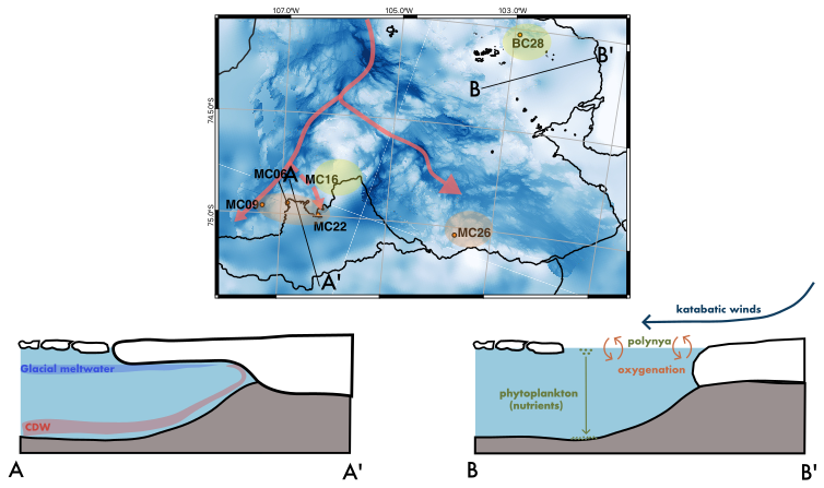
Figure 12 Summary figure of environmental conditions in the study area influencing foraminiferal populations at the sampling sites. Assumed CDW pathways in red. E. cf. exigua FP in orange and Miliammina arenacea FP in green/yellow. A to A^′ is a section across Thwaites Glacier Tongue (TGT) and the H2 former pinning point. A to A^′ is a generalization of the E. cf. exigua FP. B to B^′ is a section across Cranton Bay, illustrating the process of katabatic winds pushing sea ice away from the coast and oxygenating surface waters. In the open, phytoplankton thrives and eventually settles on the seafloor. B to B^′ is a generalization of the Miliammina arenacea FP.

The positive PC1 scores in the FA model appear to be related to the presence of CDW, and the negative PC1 scores appear to be related to glacial-meltwater-influenced modified CDW. Similar to the trend observed in the FP model, there is an increase in temperature with an increase in PC1 scores, except for the pioneer assemblage at site MC06 (Fig. 11).

PC2 correlates to the composition of the tests of the statistically significant foraminiferal species in the FA (Fig. 6). Unlike the FP model, there is no clear environmental relationship with PC2 (Fig. 11). The positive PC2 scores (quadrants I and II) contain the agglutinated species, whereas the negative PC2 scores (quadrants III and IV) contain the calcareous species (Fig. 7; Table 10).

The PCA clusters (Fig. 7b) indicate that one FA lies in quadrants I, II, and IV (Fig. 6) and is defined by CDW and calcite preservation potential (Table 1; Fig. 6). Samples from sites MC09, MC22, and MC26 are within the CDW extent and have PC1 scores greater than −5 (Tables 1, 10). Calcareous foraminifera have negative PC2 scores, and all of them comprise the statistically significant species of samples MC06, MC09, and MC26. The statistically significant and abundant species in this cluster is E. cf. exigua; thus, the FA is named E. cf. exigua FA. We suggest that the E. cf. exigua FA indicates a position of a site that is above the local CCD, partly due to CDW influence, and also the seasonal flux of phytodetritus (e.g., Gooday and Rathburn, 1999).

The second cluster in the total FA is in quadrant II and is defined by the statistically significant foraminiferal tests that are agglutinated (Fig. 6). The samples in this cluster, MC16 and BC28, have PC1 scores less than −5 and have positive PC2 scores. The most statistically significant and abundant species in the total FA from these samples is Portatrochammina spp., and therefore, it is referred to as the Portatrochammina spp. FA. Even though these two samples are located in different basins with variable glacial influence (Fig. 1), we infer that the lower sea ice cover and thus the higher phytoplankton availability affect the statistically significant foraminiferal species in this FA, with only agglutinated foraminifera and one calcareous species, Pyrgo spp., representing this cluster. The percentages of agglutinated foraminifera in the dead census are 95 % (MC16) and 55 % (BC28), respectively. The dominant calcareous foraminiferal species of BC28 are Pyrgo spp. and Globocassidulina spp., with 8 % and 4 % of the dead census and 5 % and 3 % of the live census, respectively (Tables 7, 8). The dominant calcareous foraminifera of MC16 is Globocassidulina spp. as well, accounting for 17 % of the live population and less than 1 % of the dead assemblage. Pyrgo spp. and Globocassidulina spp. have thicker test walls than other calcareous species observed in this study, which could indicate an abundant food supply. We interpret this FA to indicate higher phytoplankton availability, which allows for large agglutinated foraminifera and thick-walled calcareous foraminifera to thrive.

The main caveat of our interpretation is that there are many reasons why the other calcareous species could be less prevalent in this FA before burial. For example, a high organic carbon flux due to high productivity could produce acidic bottom-water conditions, which can be expected for both sites, especially BC28. On the other hand, site MC22, which is bathed by CDW with a temperature of 1.1 °C, is dominated by agglutinated foraminifera. Therefore, one must be cautious in interpreting a lack of calcareous foraminifera as an environmental signal.

Our work shows that it is important to study the live FAs in conjunction with in situ environmental conditions. However, to draw paleoenvironmentally relevant conclusions, preservation bias must be factored in when interpreting the total (or dead) assemblage. Living FPs provide a framework for the environmental controls on species composition of benthic foraminifera communities, aiding in the interpretation of the total FA, which also reflects what is preserved in the sedimentary record.

5 Summary and conclusions

We analyzed live and dead benthic foraminiferal assemblages in the seafloor surface sediments at six locations on the Amundsen Sea Embayment continental shelf. Four of those sites are located directly offshore of Thwaites Glacier's ice shelf front, and the two other sites are influenced by the Pine Island Polynya further east (Fig. 12). We conclude the following:

• An ice proximal live FP, E. cf. exigua FP, is largely controlled by warmer bottom-water mass characteristics and more persistent sea ice cover compared to polynya locations.

• The live Miliammina arenacea FP is associated with high phytoplankton production in seasonal open water, implying that reduced summer sea ice cover (and consequently higher plankton and, thus, food supply) exerts a strong control on the benthic foraminifera fauna at the two sites influenced by the Pine Island Polynya.

• The total census (combined live and dead) FAs are controlled by relatively warm CDW and calcite preservation. The total census E. cf. exigua FA is found above the local CCD, which is in part controlled by the presence of CDW. The total census Portatrochammina spp. FA is characterized by cooler water conditions, indicating more modified CDW.

• Ice shelf retreat signals can be observed from the foraminiferal census. At one site located at the ice shelf front of Thwaites Glacier, we observe a dramatic shift from the dead benthic FA to the live population that indicates the influence of recent ice shelf front retreat on bathymetric high H2.

• Future studies of benthic foraminiferal assemblages in the Amundsen Sea Embayment and other ice shelf front settings should aim to acquire large volumes of sediment, e.g., by dedicating more MC sub-cores to those studies, by performing multiple MC deployments at the same site, or by deploying BCs. Furthermore, we found that sediments from deep sites (>1000 m water depth) can also contain calcareous foraminifera if they are influenced by relatively warm bottom water, such as CDW. It is recommended that the samples are submerged in rose bengal for as long as possible, ideally up to several weeks (e.g., Schönfeld et al., 2012), to ensure that all live foraminifera are stained.

• Modern benthic foraminiferal assemblages from ice shelf proximal locations show that benthic ecology is sensitive to dynamic glacial changes. Along with these results, further benthic foraminifera studies from such locations will strengthen the utility of this paleoenvironmental proxy for investigating older sediments from (formerly) glaciated settings.