the Creative Commons Attribution 4.0 License.
the Creative Commons Attribution 4.0 License.
 | 04 Dec 2018
Reproducibility of species recognition in modern planktonic foraminifera and its implications for analyses of community structure
Nadia Al-Sabouni
Isabel S. Fenton
Richard J. Telford
Michal Kučera
Applications of planktonic foraminifera in Quaternary palaeoceanographic and palaeobiological studies require consistency in species identification. Yet the degree of taxonomic consistency among the practitioners and the effects of any potential deviations on community structure metrics have never been quantitatively assessed. Here we present the results of an experiment in taxonomic consistency involving 21 researchers representing a range of experience and taxonomic schools from around the world. Participants were asked to identify the same two sets of 300 specimens from a modern subtropical North Atlantic sample, one sieved at >125 µm and one at > 150 µm. The identification was carried out either on actual specimens (slide test) or their digital images (digital test). The specimens were fixed so the identifications could be directly compared. In all tests, only between one-quarter and one-eighth of the specimens achieved absolute agreement. Therefore, the identifications across the participants were used to determine a consensus ID for each specimen. Since no strict consensus (>50 % agreement) could be achieved for 20–30 % of the specimens, we used a “soft consensus” based on the most common identification. The average percentage agreement relative to the consensus of the slide test was 77 % in the >150 µm and 69 % in the >125 µm test. These values were 7 % lower for the digital analyses. We find that taxonomic consistency is enhanced when researchers have been trained within a taxonomic school and when they regularly perform community analyses. There is an almost negligible effect of taxonomic inconsistency on sea surface temperature estimates based on transfer function conversion of the census counts, indicating the temperature signal in foraminiferal assemblages is correctly represented even if only two-thirds of the assemblage is consistently identified. The same does not apply to measures of diversity and community structure within the assemblage, and here we advise caution in using compound datasets for such studies. The decrease in the level of consistency when specimens are identified from digital images is significant and species-specific, with implications for the development of training sets for automated identification systems.
- Article
(2368 KB) - Full-text XML
-
Supplement
(1264 KB) - BibTeX
- EndNote


Census counts of species abundances of planktonic foraminifera assemblages are an important means to reconstruct past sea surface temperatures (SSTs) (Kučera et al., 2005) and global diversity patterns (Rutherford et al., 1999; Niebler and Gersonde, 1998; Al-Sabouni et al., 2007). Given their low diversity and the abundance of morphological features on shells of planktonic foraminifera, it seems likely that most taxonomists will identify foraminiferal (morpho) species consistently. However, studies at a species level have shown that ecologically important species may be confused when discriminated visually (e.g. G. bulloides and G. falconensis; Malmgren and Kennett, 1977). There has never been a rigorous test of the degree of consistency among different taxonomists and of the effect of the potential differences on past environmental reconstructions and measures of community structure, such as diversity.
In a study involving Cenozoic Mediterranean planktonic foraminifera, Zachariasse et al. (1978) found that although duplicate counts made by the same person on the same samples are reproducible over shorter time periods (e.g. a few months), reproducibility over longer time periods decreases. These results indicate that taxonomic consistency could indeed be a significant source of noise in foraminiferal census counts. This issue was first explicitly highlighted by the El Kef blind test (Ginsburg, 1997a, b). The original aim of this analysis was to determine whether the Cretaceous/Palaeogene (K/Pg) extinction in planktonic foraminifera was instantaneous (e.g. Luterbacher and Premoli Silva, 1962, 1964), gradual (e.g. Herm, 1963) or step-wise (e.g. Keller, 1989; Canudo et al., 1991). Four experienced researchers were selected with profoundly different opinions on the nature of this event (i.e. from different taxonomic schools) and were given six identical unprocessed samples from above and below the K/Pg boundary, without prior knowledge of their relative stratigraphic position. They were asked to determine the nature of the extinction event. The results showed an enormous divergence in the results by the four participants (species richness varied between 45 and 59 in the Maastrichtian samples with only 16 species names shared by all four participants). However, evaluating the wider relevance of this result is hampered by differences in sample-processing procedures among the participants and the known controversy in the taxonomy of that time period. Additionally participants were not working on the same specimens, making it hard to determine which of these factors was more important (Ginsburg, 1997a, b). Although no authoritative conclusions could be reached, this experiment revealed a pressing need to implement more rigorous quality control mechanisms in planktonic foraminiferal studies, as is increasingly the case in other fields of micropalaeontology (e.g. Kelly et al., 2002; Weilhoefer and Pan, 2007).
The implications of taxonomic disagreements could be especially relevant when analyses are performed on large datasets collected by multiple workers. In many cases, such studies are based on compilations of counts conducted by different researchers (e.g. CLIMAP, 1976; Kučera et al., 2005; Rutherford et al., 1999). For example, census counts of planktonic foraminifera are used in Quaternary palaeoceanography as an input in transfer functions for quantitative palaeotemperature estimates. The CLIMAP group went to great lengths to standardise sampling practice in producing counts of Quaternary planktonic foraminifera assemblages (Imbrie and Kipp, 1971; CLIMAP, 1976). As a result, counts of planktonic foraminifera for transfer function are typically based on 300 specimens and fewer than 30 species, with several of the counted categories including more than one species. Despite this, there is no guarantee the taxonomic concepts used by the different workers will be the same. Similarly, there is evidence that diversity metrics are sensitive to the sampling protocols used to collect the data (Al-Sabouni et al., 2007), which may vary across these large datasets. They are also likely to be influenced by the taxonomic concepts, but this has yet to be studied. Therefore, it is imperative to determine the extent of taxonomic discrepancies in the identification of Quaternary planktonic foraminifera and to assess the impact such discrepancies may have on commonly used palaeoceanography tools or diversity metrics.
Recently there have been a series of studies reporting on attempts to develop automated image analysis and identification tools from images of planktonic foraminifera (Hsiang et al., 2016; Ranaweera et al., 2009a, b; MacLeod et al., 2010; O'Neill and Denos, 2017; Zhong et al., 2017). Work on other plankton groups has found that agreement varies significantly, with averages of around 70 % (Simpson et al., 1992; Culverhouse et al., 2003). It has been recognised that images do not necessarily capture all the features that participants use in identification, so obtaining accurate species level identifications from them could be more challenging (Culverhouse et al., 2003; Austen et al., 2016; Zhong et al., 2017). Many of these systems rely on a training dataset produced by one or more scientists using digital images. In the context of developing these training datasets, it is therefore important to determine how the taxonomic consistency of identification of planktonic foraminifera compares between workers when using actual specimens or digital images.
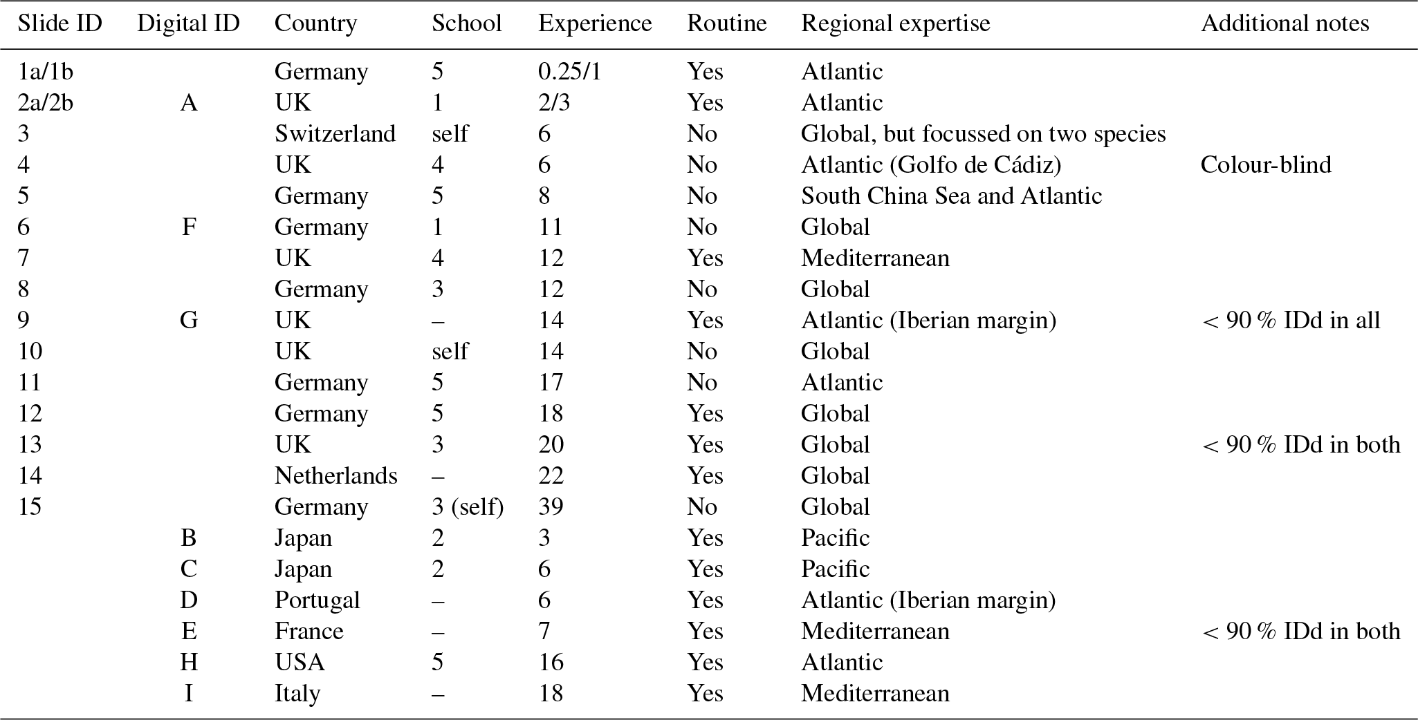
Table 1Participant details and background information for the slide (numbers) and digital (letters) tests. Participants 1 and 2 conducted duplicate counts on the slide test, separated by 1 year (a and b). The digital test by participant 2 was conducted after 3 years (i.e. equivalent to 2b). In the school column, “–” indicates that the participant was the only member of the school represented in this analysis, but they were not self-taught (for more details on the taxonomic schools, see Supplement Fig. S1). Experience is measured in years. All participants identified all the specimens from both size fractions. The “Additional notes” column includes factors that may have affected the results, for example where fewer than 90% of specimens were identified (IDd).
In this study, we present the results of an experiment which (1) determines the taxonomic disparity amongst a set of researchers with different level of experience and (2) investigates the impact of the observed taxonomic inconsistencies on temperature and community structure estimates. Furthermore, we (3) examine the effects on taxonomic consistency when using digital images of specimens as opposed to the actual specimens, thus simulating the potential information loss in automated image analysis training datasets.
2.1 Selection of specimens
The specimens used in this analysis were collected using a box corer at a depth of 1940 m, from the North Atlantic subtropical core top sample GIK 10737 (30.2∘ N, 28.3∘ W). The foraminifera exhibit no signs of dissolution. This site was selected for its high diversity (following Al-Sabouni et al., 2007) to produce an assessment of the taxonomic concepts of the majority of late Quaternary planktonic foraminiferal species.
The sample was initially split into two separate halves using a microsplitter. One half was sieved to include all specimens >125 µm, which is more appropriate for diversity analyses in Holocene planktonic foraminifera (Al-Sabouni et al., 2007). The other half was sieved for specimens >150 µm as this is the most commonly used sieve size for planktonic foraminifera studies (e.g. CLIMAP, 1976) and is required for estimating sea surface temperatures (SSTs) using transfer functions (Kučera et al., 2005). Both of the sieved aliquots were further split until ∼300 specimens remained. From these, a representative 300 individuals were selected and fixed in place on slides. The taxonomically more informative umbilical side was typically oriented upwards, although this was not possible for all species. Fixing the specimens prevented participants from viewing them from multiple angles (unlike a normal census count), but it ensured the specimen order was not altered and no specimens were lost during slide manipulation. Each specimen was then photographed, for use in the digital test, and the maximum diameter was measured using ImageProPlus 6.0.
2.2 The participants and test procedure
Two versions of the identifications were set up: (1) the slide test using the actual (glued) specimens and (2) the digital test using the images of those same specimens; so, with the two size fractions for each, there were four sample sets. Each participant was asked to identify all 300 specimens of both size fractions for their chosen test type. The only criterion for selection in the analysis was that the participant had conducted counts on Holocene planktonic foraminifera at some stage in their career. However, owing to the risk of specimens becoming dislodged, participants of the slide test were restricted to western Europe. The slide test was completed by 15 taxonomists representing more than eight taxonomic schools, whose length of experience ranged from 3 months to 39 years (Table 1). Taxonomic schools were defined based on the participant's main teacher of taxonomy and who the teacher, in turn, was taught by (see Supplement Fig. S1). As far as it is possible to ascertain, there is little connection between the taxonomic training of the main teachers in the schools. Nine taxonomists participated in the digital test, representing three additional taxonomic schools (Table 1; Supplement Fig. S1) and a more global distribution. Three participants completed both the slide test and the digital test. Two participants conducted duplicate counts for the slide test separated by a year.
Each participant was given instructions for the counting procedure and described the length of their experience, the source of their taxonomic training and their areas of expertise (Table 1). Participants were asked to follow (morphological) taxonomic concepts based on Hemleben et al. (1989), although G. tenella and G. rubescens (white) were grouped. (The only way to distinguish these is by the presence of a secondary aperture on the spiral side of the shell in G. tenella. As this side was not visible in the mounted specimens, the white specimens of both were grouped under G. rubescens (white)). Participants were provided with a list of species names (see Supplement, Sect. S1). The use of reference books was permitted if participants so desired, but conferring with another person was not. This was ensured either by the experiment designer's presence during the test or by a contract signed by the participant agreeing to that point. While the participants were encouraged to identify all specimens, they could leave some unidentified. The choice of microscope and the magnification to study the slide specimens was left to the discretion of the participants.
2.3 Analyses
Theoretically, the analysis of the individual identifications should be carried out against an objective “known” identity of the specimens. In reality, this cannot be achieved on empty shells as they do not contain DNA for genetic analysis. Instead, we used the participants' identifications to derive an “authoritative” consensus identification for each specimen. When there is 100 % agreement between all participants, then the consensus is clear. The “strict consensus” is calculated based on more than 50 % of the participants agreeing on an identification, with the remaining specimens being classified as having “no consensus”. However, the latter occurred too often, so where fewer than 50 % of participants gave the same answer, we determined a “soft consensus” based on the most frequent identification. Where multiple names had the same frequency, the alphabetically first species name (based on the abbreviations) was used. A sensitivity analysis was done to investigate the impact of alternatively classifying these specimens as “no consensus attainable”. As the slide and digital tests for a given size fraction were based on the same specimens, for all of the analyses except the comparison between the slide and digital results, these three different consensus identifications were obtained from the combined results of both tests. Soft consensus identifications (hereafter referred to as consensus IDs) defined in this way were obtained for all specimens for each size fraction.
In order to determine the disparity among the researchers in these different tests, the percentage agreement was calculated as the fraction of identifications that agreed with this consensus ID. To ensure differences in percentage agreement between the slide tests and the digital tests were not influenced by the number of participants, the slide-test results were subsampled to contain the same number of participants as the digital test (i.e. nine). This subsampling was repeated 1000 times, and the consensus estimates were then recalculated with these subsampled datasets to obtain percentage agreements that could be compared. Confusion matrices were calculated to visualise which species were most frequently misidentified, using the R package “caret” (Kuhn, 2018). These show how the identifications given to a specimen compare with its consensus ID. They highlight which species concepts are most consistently applied. The influence of size on the accuracy of the identifications at a specimen level was also investigated.
To visualise the similarity in the identifications among the participants, the ordination of pairwise distances was plotted using non-metric multidimensional scaling (NMDS). This multivariate method orders participants by the rank distance between their pairwise identifications; participants that plot closely together are more similar to each other in their identifications than those that plot further apart (Hammer and Harper, 2008). Gower distances were calculated using the function “daisy” in the R package “cluster” (Maechler et al., 2015), which can calculate distances using nominal data. Two NMDS analyses were created, one for each size fraction. For both analyses, the participants' identifications for each specimen of both the slide tests and the digital tests, as well as the consensus ID values were included. The NMDS plots were run using the package “vegan” (Oksanen et al., 2015). The number of dimensions was chosen as the minimal number of dimensions with a stress less than 0.2 (following Clarke, 1993). To test whether identifications were more similar within taxonomic schools, the distances between participants within each school were compared to those between schools for both the slide and the digital tests.
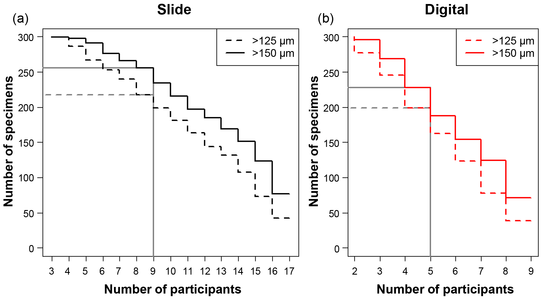
Figure 1A plot of the minimum number of participants that agreed on an identification for each specimen, split by each analysis. For example, in the slide test all 300 of the specimens had at least three people agreeing on an identification. There were 17 participants in the slide test (a), as two took the test twice, and 9 in the digital test (b), so those values in each represent the number of specimens that had complete agreement in their IDs. The grey lines indicate where the strict consensus would be for the separate consensus estimates, with more than half of the participants agreeing on the answer (although the strict consensus and the consensus ID used in most of the analyses were calculated from the combined slide and digital datasets).
To assess the impact of taxonomic inconsistency on transfer functions, the census counts on the >150 µm fraction were converted into annual mean SST estimates (10 m water depth), using artificial neural networks (ANNs) trained on the North Atlantic MARGO calibration dataset (Kučera et al., 2005). (This method has been calibrated for the typical abundances observed in the >150 µm size fraction.) The transfer function analysis does not include all the species and G. menardii is merged with G. tumida (for more details, see Supplement, Sect. S1). These estimates were compared with the modern annual mean SST at that site for 10 m water depth taken from the World Ocean Atlas (Antonov et al., 2008). To determine the influence of inconsistency on the community structure estimated from a sample, three diversity measures – species richness, Shannon–Wiener and dominance (measured as Simpson's diversity, D) – were calculated for each of the participant's assemblage counts and compared to the estimates based on the consensus IDs. These were additionally compared to the range of values observed in the Atlantic as a whole, using data from Siccha and Kučera (2017).
To investigate the differences between the slide and digital-test results, the consensus values were recalculated separately for these two types for each size fraction. The percentage agreements with these separate consensus identifications could then be compared to the estimates based on the joint consensus. Sensitivity analyses were run to test whether the number of specimens identified as “no consensus” was influenced by the number of participants involved in the separate tests; the slide-test participants were subsampled 1000 times to contain the same number of participants as the digital test (i.e. nine), and the strict consensus was recalculated. Confusion matrices were plotted using the strict consensus values, to determine where confident identifications differed. All analyses, with the exception of the calculation of the SST estimates, were carried out using R version 3.2.3 (R Core Team, 2015).
3.1 Participant agreement
The number of specimens in each of the four tests with complete agreement in their identification ranged from 38 (12.7 %) for the >125 µm digital test to 77 (25.7 %) for >150 µm slide test (Fig. 1). In the majority of analyses in this paper (i.e. excluding the slide/digital comparisons), the consensus estimates were calculated on the combined slide/digital results; there, 100 % agreement was only reached for 24 specimens (8 %) in the >125 µm size fraction and 46 specimens (15.3 %) in the >150 µm split. When the strict consensus of 50 % agreement was used, this increased to 209 (69.7 %; >125 µm) and 237 (79 %; >150 µm). However, that still left a significant fraction of the 300 specimens without a consensus. To provide a soft consensus ID for every specimen, the level of agreement was sometimes as low as 19 %. The number of specimens where multiple names were equally common (so the consensus was chosen alphabetically) was only five for the >150 µm dataset and six for the >125 µm size fraction. Examples of the digital images of each species for specimens with high and low agreement levels are shown in Supplement Sect. S4. The full image collection is available in the supplementary data provided in Fenton (2018).
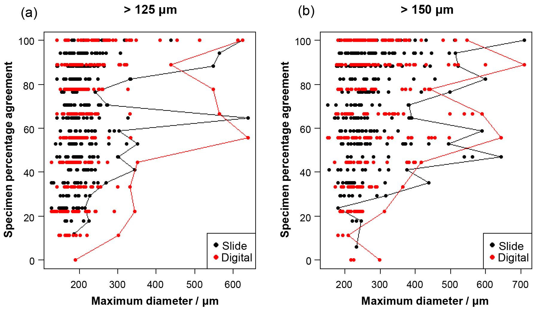
Figure 2The influence of size (maximum diameter) on the maximum agreement of the identification of a specimen, split by slide/digital test. Agreement of 100 % implies all participants in that test agreed with the consensus ID. The maximum size for each level of agreement is indicated by the line. For comparison, Supplement Table S3 has the maximum observed diameter of the specimens for the species in this analysis.
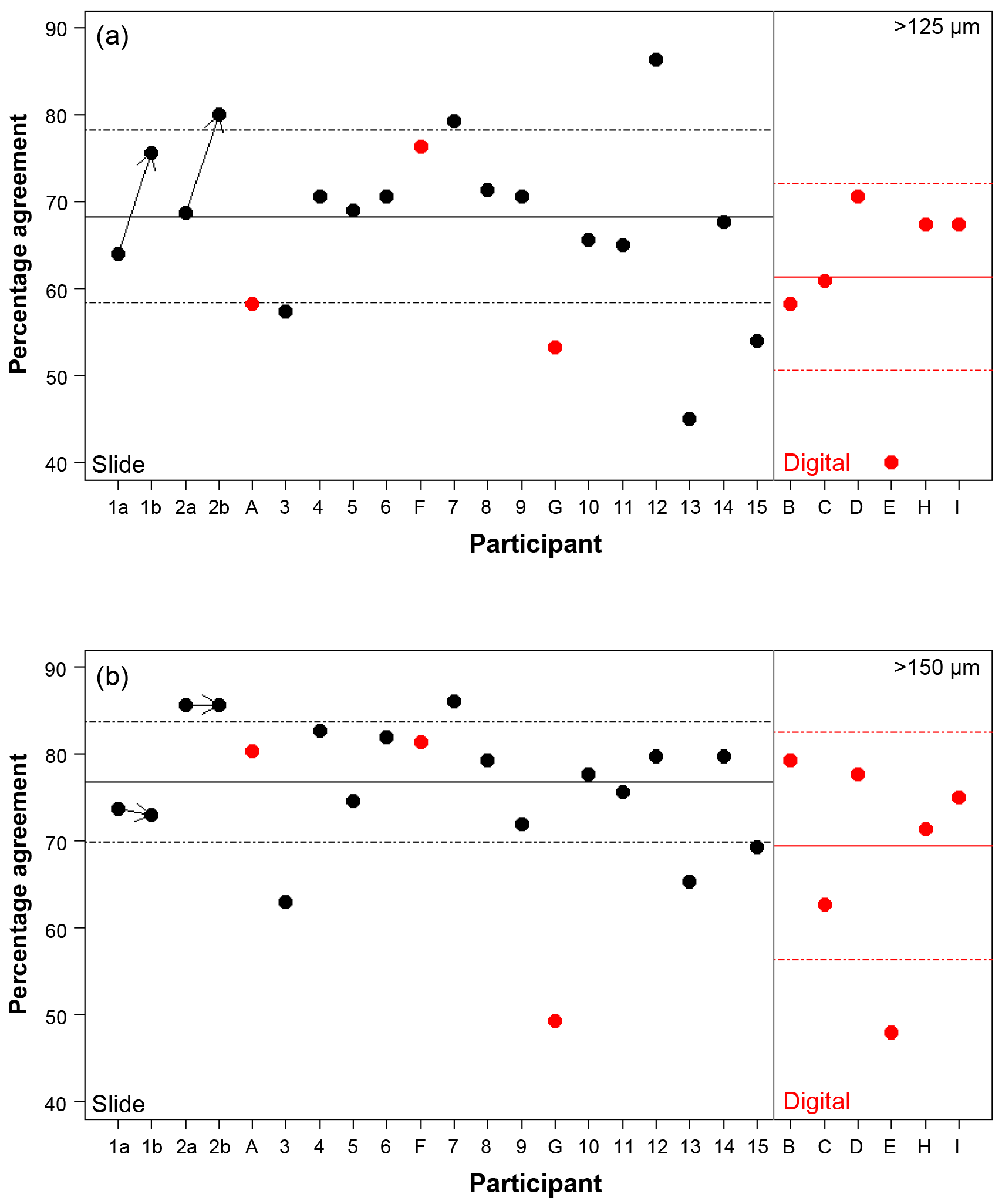
Figure 3The percentage agreement in the taxonomic identification between each participant and the consensus ID, shown separately for the different size fractions. Exact agreement with the consensus would be implied by 100 %. Participants are ordered by slide (numbers, black)/digital (letters, red) and then by experience, so the left side shows the least experienced participants. The three participants that performed both the slide and the digital tests are plotted together for comparison. The paired results for the participants who repeated the analysis after additional training are joined by an arrow. The solid line is the mean, and the dashed lines show 1 SD. Note the two graphs have the same scale.
Specimen size has an unexpectedly weak influence on the level of agreement (Fig. 2), although larger specimens in both analyses are generally more likely to be identified consistently. Even though agreement is higher for specimens larger than 300–400 µm, with most such specimens getting a strict consensus identification, it is still possible for specimens as small as 140 µm to obtain 100 % agreement values. (Most of the specimens in the >125 µm analysis are less than 300 µm.)
Using the consensus ID, the percentage agreement by a participant with that ID can then be investigated (Fig. 3; Table S1). This ranges from 40.0 % to 86.3 %, with the lowest agreement being found in the >125 µm digital test and the highest in the >125 µm slide test. The mean values were approximately 8 % lower in the >125 µm fraction compared to the >150 µm fraction in both tests (68.3 % vs. 76.8 % for the slide test and 61.4 % vs. 69.4 % for the digital one; Fig. 3). Similarly, the level of agreement among the participants in the digital test was 7 % lower compared to the slide test (Fig. 3). The higher number of participants in the slide test did not qualitatively alter these results (see the subsampled comparisons in Supplement Fig. S2). The standard deviation in an individual's percentage accuracy with these subsampled consensus values was 1 % at the maximum. If specimens with ties were designated “no consensus attainable”, then the mean values were very slightly lower, and there are only small changes in the individual participants' scores. There appears to be no strong signal of length of experience on accuracy (higher numbers/later letters indicate participants with more experience; Table 1; Fig. 3). Routine counting slightly raises the percentage agreement of the participants for the slide test (there is insufficient data for the digital test as only one worker was classified as not a routine counter; Table 1).
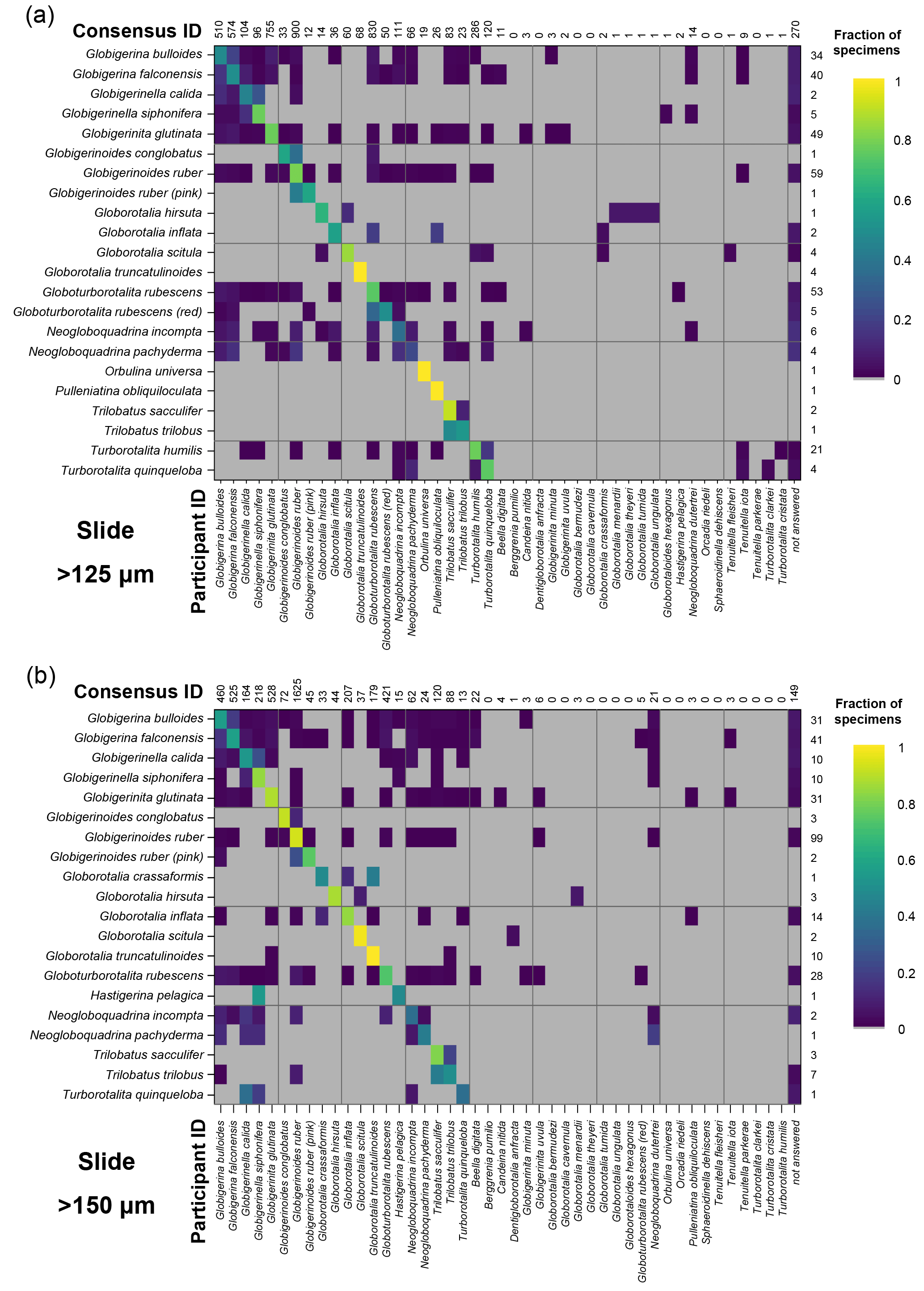
Figure 4Confusion matrices for taxonomic identifications in the two slide tests. The y axis shows the consensus ID, and the x axis shows the names given by the participants to the individual specimens. Where a specimen was always identified correctly, only one square in that row would be filled, indicating the fraction of specimens correctly identified is 1. The numbers along the top indicate the number of specimens given that name in the analysis. The numbers at the right indicate the number of specimens of each species in the consensus ID. The digital results are shown in Supplement Fig. S3; the versions with the ties classified as “no consensus attainable” are in Supplement Fig. S4. Numerical versions are available in the supplementary dataset (Fenton, 2018).
The confusion matrices highlight the species concepts which are least prone to disagreement (see Fig. 4 for the slide test; the digital results, in Supplement Fig. S3, are broadly similar). There were clearly large and systematic differences among species. Nearly everyone agreed upon the identification of some species (e.g. G. truncatulinoides, P. obliquiloculata, O. universa). For other species the disagreement was very high (e.g. N. pachyderma). Some of the disagreements indicate “pairwise” differences between two closely related species or species concepts (e.g. T. sacculifer and T. trilobus, or G. siphonifera and G. calida), whereas in other cases (e.g. G. falconensis) the alternative identifications cover a wide range of species. It is important to note that these results are most robust for frequently occurring species (indicated by the column of numbers on the right of Fig. 4). Using the alphabetically first species to split ties in the consensus determination makes the agreement for a couple of species, e.g. G. bulloides, appear slightly worse than if specimens with ties are designated as “no consensus attainable” (Supplement Fig. S4), but there are few other changes.
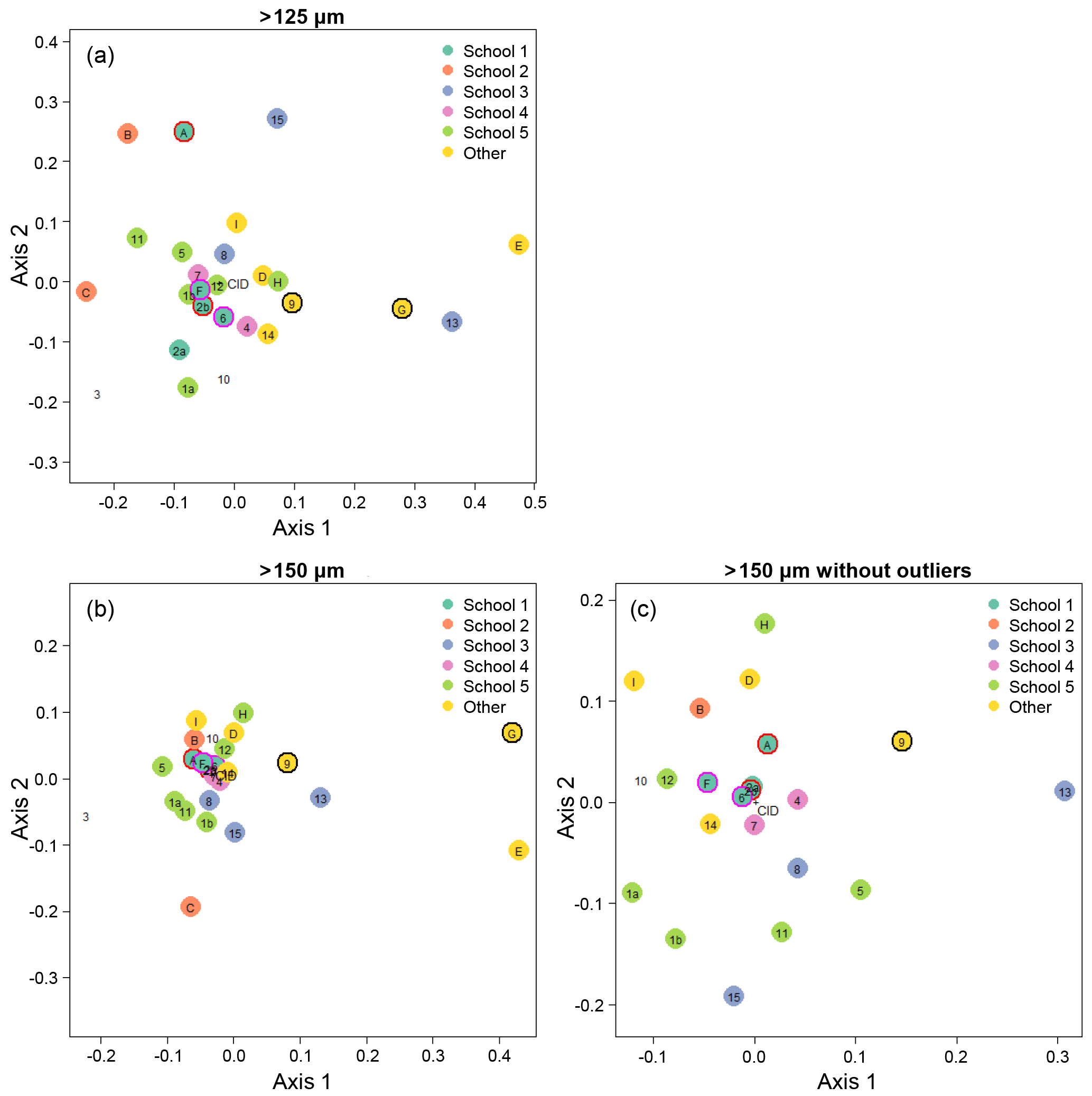
Figure 5Visualisation of the taxonomic agreement among the participants using non-metric multidimensional scaling (NMDS) plots for the different size fractions. Panel (a) shows the >125 µm size fraction. The more extreme outliers in the >150 µm plot (b) makes the placement of the main cluster of points less robust. To overcome that problem, the >150 µm NMDS was rerun with the most extreme points removed (c). As elsewhere, numbers indicate the slide test; letters indicate the digital test. Colours indicate attribution to a taxonomic school; “other” indicates schools with only one individual. Unfilled points are self-taught individuals. (For more details on the taxonomic schools, see Supplement Fig. S1.) Outlined circles highlight paired analyses. Also shown is the position of the consensus ID (CID).
We determined that 2 dimensions were sufficient for an NMDS to describe the complexity of the data, based on a stress value of <0.2 (Clarke, 1993); the NMDS plots are shown in Fig. 5. Two NMDS analyses were run for the >150 µm size fraction, as the more extreme points reduce the accuracy of the placement of the central points; Fig. 5b is the full dataset, and Fig. 5c has the four most extreme participants (3, C, E, G) removed. Participants who identified fewer than 90 % of the specimens (9, 13, E, G; Table 1, Table S1) tend to plot further from the consensus. The duplicate analyses on the slide test (1a/1b, 2a/2b, indicated by outlined circles) tend to plot close together, although this is more pronounced in the >150 µm size fraction (Fig. 5c). The slide vs. digital analyses of 2b/A and 6/F are close in the >150 µm analysis but more disparate in the >125 µm analysis. 9/G are separated in both. Analysis of the pairwise distances between points indicates that generally identifications by people within the same school plot closer together than those between schools. Identifications based on slides tend to be more similar than those based on digital tests both within and between schools, although this effect is more pronounced for the smaller size fraction (Supplement Fig. S5). However, as there are only two schools in the digital tests that have more than one participant, these results are only indicative. Some schools (e.g. School 1, School 4) show more consistent clustering than others. Self-taught individuals (those without filled circles in Fig. 5) are more likely to have distinct taxonomic IDs, rarely plotting close to the consensus values.
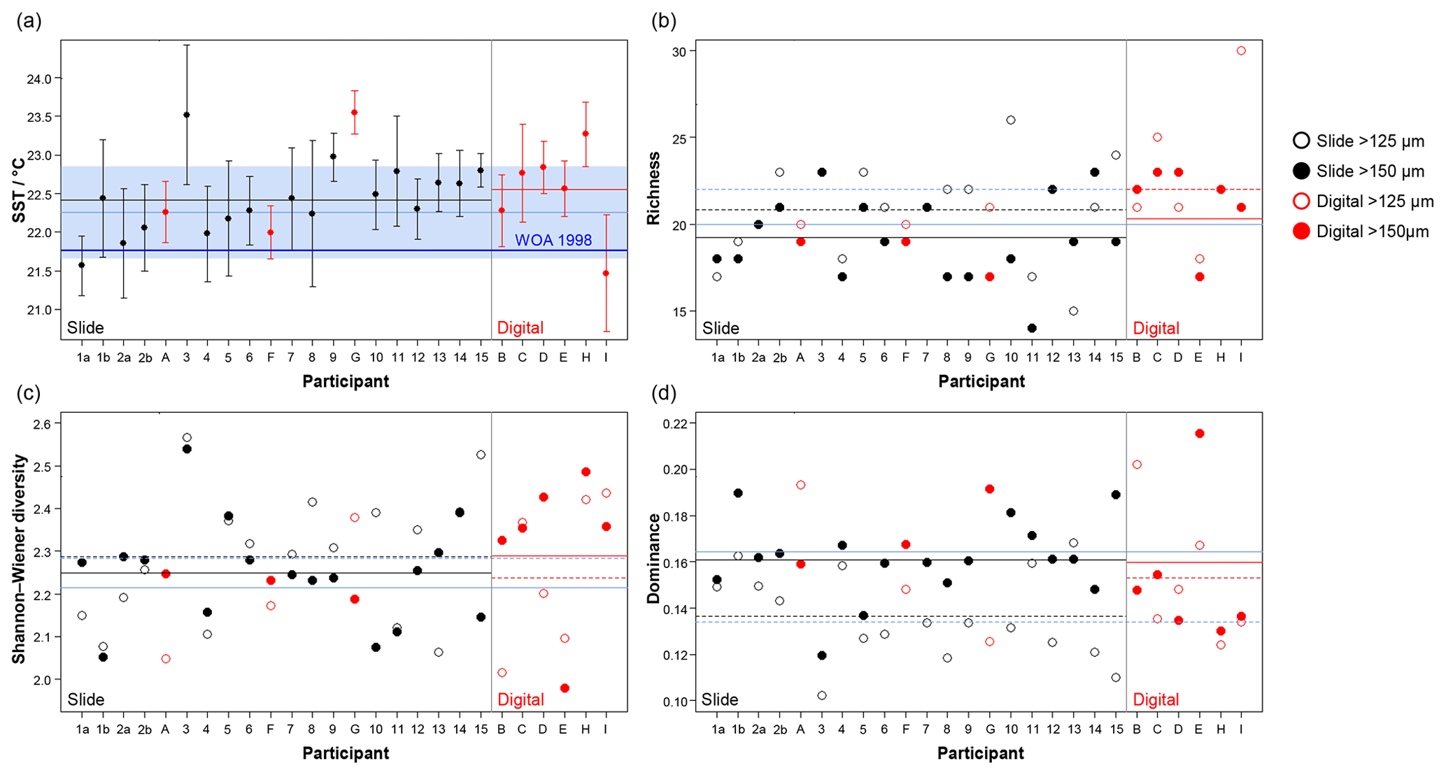
Figure 6Transfer function temperature reconstructions (a) and community structure (b, richness; c, Shannon–Wiener diversity; d, dominance) estimates for assemblage counts from the four analyses. The black/red lines indicate the mean values for the slide/digital tests and the (thin) blue is the consensus estimate: solid line >150 µm; dashed line >125 µm. The order of participants is the same as in Fig. 3. The error bars in (a) show 1 standard deviation among the 10 temperature estimates derived from the ANN technique (see Kučera et al., 2005); the 1 standard deviation for the consensus is indicated by shading. The World Ocean Atlas value (thick blue line) is added for reference. Note temperatures were only calculated for >150 µm. (These figures are shown separated by size fraction in Supplement Fig. S6.)
3.2 Effects on temperature and diversity estimates
The slide-test and the digital-test mean SST estimates are similar (22.4 and 22.6 ∘C; Fig. 6a, Table S2), although the digital-test results are more variable. The WOA (World Ocean Atlas; Antonov et al., 2008) annual SST for the location of the analysed sample, 21.76 ∘C, is ∼0.5 ∘C lower than the consensus (22.3 ∘C) and the mean estimates and thus well within the ∼1 ∘C prediction error of the method (Kučera et al., 2005). Eight participants plot outside this 1 ∘C range, but only two (G and H) do not overlap with their (1 SD) error bars. These two have lower counts of cold-water taxa (including G. bulloides and G. falconensis) and higher counts of warm-water species (e.g. Globigerinoides ruber (pink)). Additionally G has the highest count of unidentified specimens.
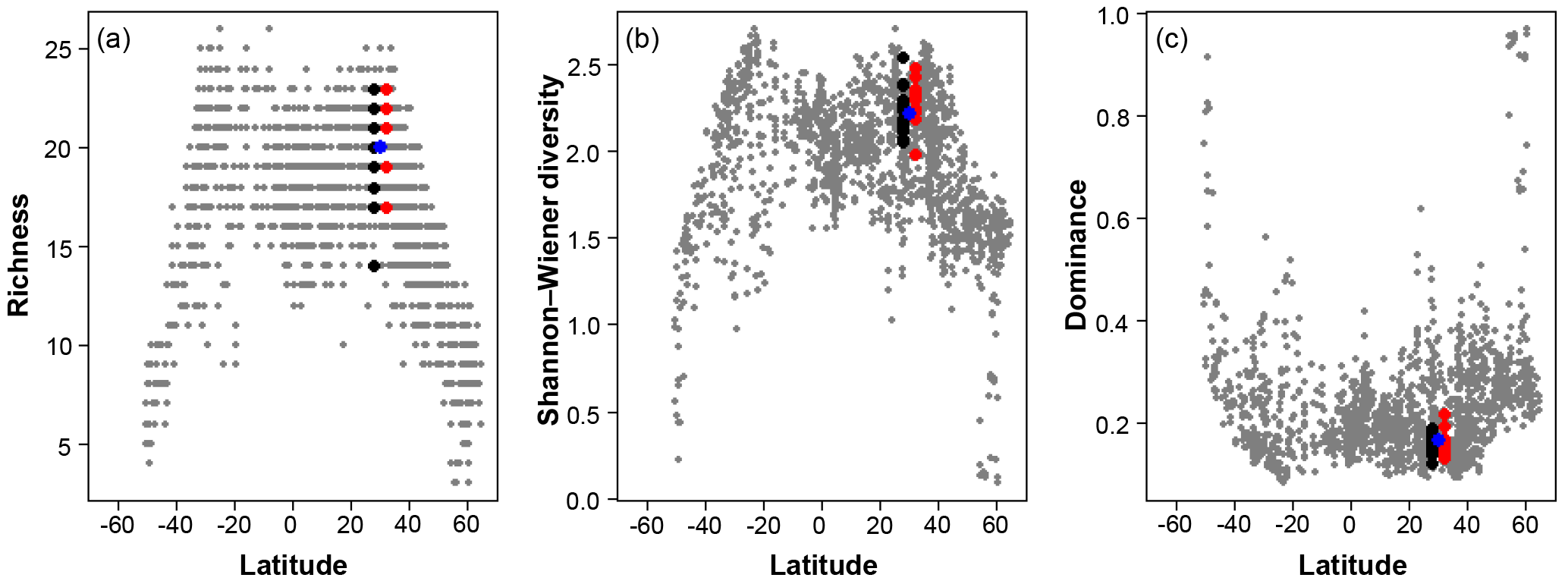
Figure 7A comparison of the three diversity metrics (a, richness; b, Shannon–Wiener diversity; c, dominance) with the range of values observed in the Atlantic Ocean. The blue points indicate the consensus estimate. Black/red points indicate the participant data from the slide and digital tests (respectively) of the >150 µm size fraction in this analysis; they are offset slightly from the true latitude for clarity. Grey points are data for the Atlantic Ocean taken from ForCenS (Siccha and Kučera, 2017).
The community structure metrics show a larger amount of variation around the consensus values (Fig. 6b–d, Table S2). The richness of the >150 µm is typically lower and abundances are more even with fewer rare species than the >125 µm fraction. Slide analyses tend to have lower richness (Fig. 6b), although the three workers who performed both the slide test and the digital test mostly show the opposite trend, with a less diverse digital dataset. For the richness analysis, the digital estimates are closer to the consensus values for both size fractions although there is a lot of spread; for the abundance-based Shannon–Wiener and dominance metrics (Fig. 6c, d), the slide estimates are closer. As the actual diversity in each sample (i.e. for each size fraction) is the same, these diversity indices highlight the different taxonomic concepts of the participants. The comparisons for each metric with the Atlantic data from the ForCenS dataset (Siccha and Kučera, 2017) are shown in Fig. 7. The consensus values tend to be in the middle of the range expected at that latitude, but the participants' individual results show a broad spread, covering much of the range of variation observed for the given latitude in the ForCenS dataset. This spread is most pronounced for the richness.
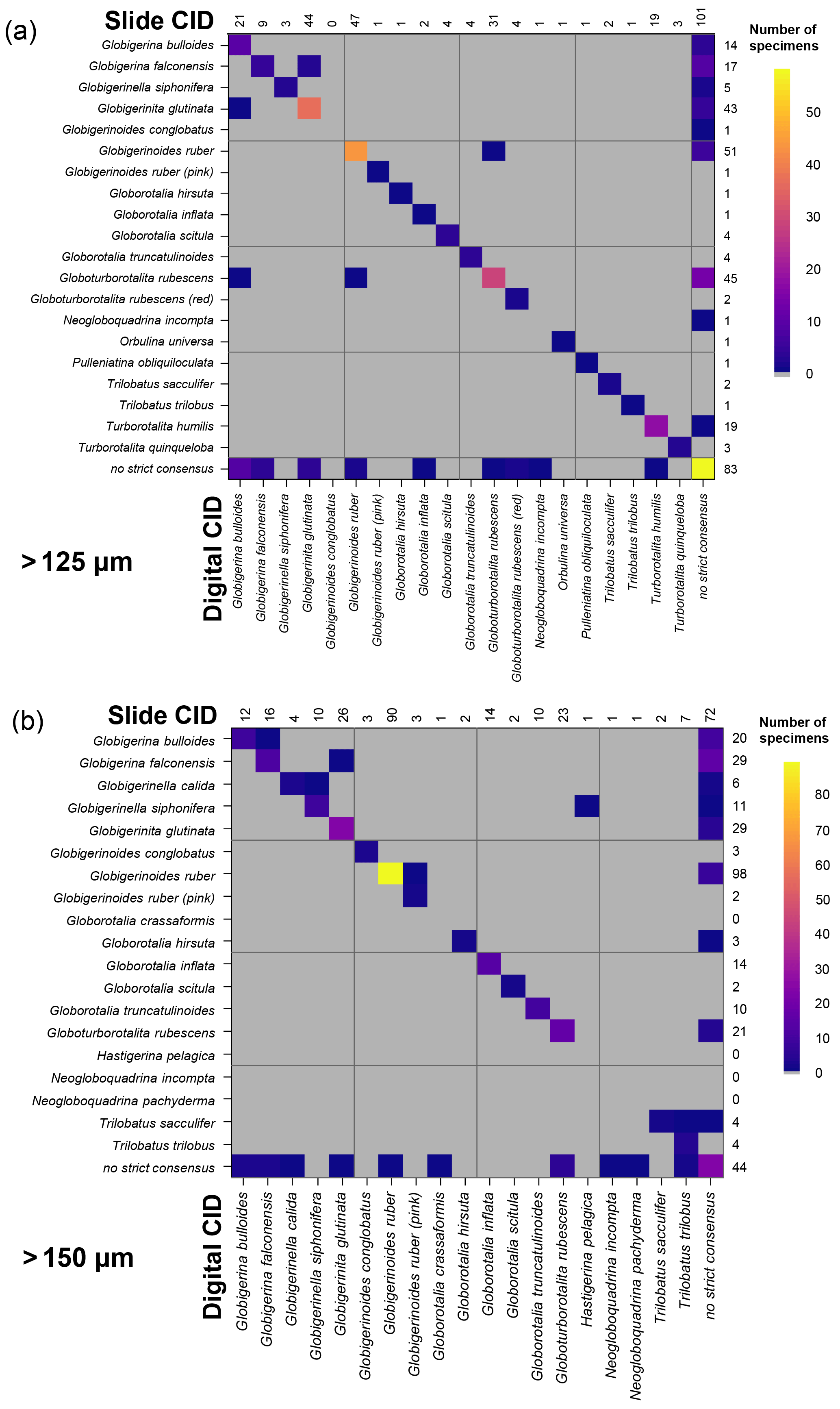
Figure 8Confusion matrices showing the comparison between the slide and the digital strict consensus values, if they are calculated separately, for the two size fractions. The y axis shows the slide consensus ID, and the x axis shows the digital consensus ID. Where both agree on all the specimens of a species, only one square in that row/column would be filled. NB: the colouring on these indicates the number of specimens rather than the fraction correct. The values indicate the number of specimens of each species in each consensus. Supplement Fig. S8 has the versions of this figure for the soft consensus and for where ties are designated “no consensus attainable” rather than based on alphabetical order. Numerical versions of these confusion matrices are available in the supplementary dataset in Fenton (2018).
3.3 Slide vs. digital
When the consensus values are recalculated separately for identifications in the slide and digital tests using the strict consensus, then those specimens that are given names in both the slide and the digital tests have very high agreement (96 %–97 %). However, these specimens only constitute 58 % of specimens at >125 µm and 69 % of specimens at >150 µm. When the unidentified specimens are included in the comparison (as “no consensus”) the agreement drops to 75 % for both size fractions. The digital tests have roughly twice as many specimens that are unidentified in the strict consensus but are identified in the slide tests (>125 µm: 43 in digital, 25 in slide; >150 µm: 48 in digital, 20 in slide). (These results hold when a subsample of the slide data is used so that both analyses have equal numbers of participants; Supplement Fig. S7.) With separate soft consensus IDs, 78 % of the identifications are the same between the slide tests and the digital-test results for the >125 µm size fraction and 83 % in the >150 µm size fraction. This use of separate consensus IDs also makes the mean agreement of the digital tests appear only >5 % worse than the slide tests rather than 7 % seen with the combined consensus.
The confusion matrices comparing these two sets of strict consensus values indicate which specimens are identified confidently in the slide and digital tests (Fig. 8). These show that there is relatively little disagreement for specimens that are identified by a majority of participants in both the slide and the digital tests. However, the digital test has more specimens that do not have a majority, particularly for those identified as G. bulloides, G. falconensis and G. rubescens in the slide tests. Supplement Fig. S8 shows these matrices for other methods of estimating the consensus.
Three participants (A/2b, 6/F, 9/G) conducted comparative counts of the slide and digital tests (Table 1). Agreement between their slide and digital identifications ranged between 57 % (A/2b>125 µm) and 77 % (A/2b>150 µm and G/9>125 µm). For two of these comparisons the >150 µm size fraction was more similar, although for G/9, it was 6 % less similar. In five of the six cases the agreement of the slide tests with the consensus ID was higher than their comparable digital tests (Fig. 3).
4.1 Sources of taxonomic inconsistency among researchers
When specimens from a representative >150 µm split of a tropical sample are fixed in place, the participants in this analysis on average only obtained 75 % agreement with a consensus estimate; for >125 µm this value drops to 68 %. The highest agreement of any individual with the consensus is only 86 % of specimens, although that does not necessarily mean that only 86 % of the specimens were identified “correctly”. The method used to obtain the consensus identifications in this analysis do not necessarily produce the “true” identification (in terms of genetic species) although it is the most objective answer that can be obtained from this analysis. If participants were able to communicate and explain their identifications, then it is likely that some of these consensus estimates would be considered incorrect, especially those that only have a low majority agreement. That might raise an individual's accuracy, although it would not have a large effect on the mean value because a change in the consensus ID always leads to a trade-off between higher consistency for some participants and lower for others.
Based on the associated metadata that were collected as part of this analysis, we can identify a set of correlates of lower agreement. Unsurprisingly, those participants who left many specimens unidentified tended to have a lower agreement with the consensus. Similarly, those who do not regularly perform community counts tend to differ more. Generally, self-trained taxonomists were more likely to disagree with the community consensus, producing estimates that were more marginal in NMDS space (Fig. 5). There is some evidence that identifications are more similar within taxonomic schools, for both the slide and digital tests (Fig. 5; Supplement Fig. S5). The results of Fenton et al. (2018) tend to support this conclusion, with the four more experienced workers achieving median agreements of 79 % for an analysis of the >125 µm size fraction, which is relatively high compared to the results in this analysis. These four all came from the same taxonomic school, and the consensus IDs were obtained from the main teacher of that school. However, larger samples from multiple taxonomic schools would be required to test this conclusion explicitly, particularly for the digital tests where only two schools have more than one member. If this result is true, it indicates that individual teachers can influence the taxonomic concepts used in an analysis, which would contribute to the differences observed across the planktonic foraminiferal community as a whole. Community taxonomic projects like the Palaeogene atlases (Olsson et al., 1999; Pearson et al., 2006; Wade et al., 2018), where members of multiple taxonomic schools come together to discuss concepts, are likely to be a useful way of overcoming these differences. These results suggest that taxonomic training and revision of species concepts before performing community counts are likely to be important for taxonomic consistency.
Length of experience does not correlate with a higher agreement (Fig. 3 – higher numbers/letters indicate more experience). Even those participants who had been working with planktonic foraminifera for less than 5 years (1, 2) obtained accuracies that were similar to the others. The two participants who repeated the identification after additional experience showed an improvement with time in the >125 µm size fraction, although there was little change in the >150 µm size fraction (Fig. 3). The participant with more experience (2) showed greater similarity between their two counts (80 % in the >125 µm fraction and 96 % in the >150 µm fraction, compared with participant 1's results of 61 % in the >125 µm fraction and 68 % in the >150 µm fraction). This individual reproducibility, at least for participant 2, is similar to that found by Zachariasse et al. (1978). In the >150 µm fraction, participant 1 identified the same number of specimens in agreement with the consensus (∼74 %) each time but traded the consistency in species identifications of some species, including G. falconensis and G. siphonifera, in the first count for a consistency in the classification of others, e.g. G. bulloides, G. rubescens and G. ruber, in the second count. These results suggest that during the initial stages of taxonomic training, accuracy may increase rapidly, but other than that there is no obvious relationship of accuracy with length of experience. The improvement is likely to be a result of further taxonomic experience/training obtained by these participants during this time period. Analysis by Fenton et al. (2018) supports the conclusion that with less than 1 year of training, high accuracies can be obtained, although they find there is still a signal of experience on accuracy for foraminiferal workers with up to at least 4 years of experience. Their results also highlight that regular revisions of taxonomic concepts for participants who are performing community counts, irrespective of how long they have been working, are likely to be beneficial.
4.2 Ambiguous species and common misclassifications
The results of our experiment reveal that in the case of planktonic foraminifera, taxonomic misidentifications have some predictable features. Some species (e.g. Globorotalia truncatulinoides, Orbulina universa) are consistently identified the majority of the time; other species concepts (e.g. Globigerina bulloides, Neogloboquadrina pachyderma) have more disagreements (Fig. 4). The disagreements shown in the confusion matrices (Fig. 4; Supplement Fig. S3) highlight the species concepts that would particularly benefit from improved references and future taxonomic efforts. Often confusion occurred between morphologically similar species (Hemleben et al., 1989). This raises the possibility that, were the participants able to see the specimens from multiple perspectives, then the taxonomic consistency might be higher than what is observed in this experiment. There is a suggestion of this in Fenton et al. (2018), where, for example, G. conglobatus (which has a distinctive spiral side) has higher accuracy, although this is not explicitly tested. In many cases species confusions even occurred between different genera (Fig. 4), suggesting that attempting to solve this problem by grouping phylogenetically related species/forms (e.g. T. trilobus and T. sacculifer) will only remove a subset of the disagreements. Additionally, unless foraminiferal workers have kept up to date with the latest taxonomic papers, then their taxonomic concepts will not match current thinking. In planktonic foraminifera, this is exacerbated by the lack of a modern authoritative taxonomy. The main reference has been for many years Hemleben et al. (1989), the focus of which was not taxonomy, and alternative references, such as Kennett and Srinivasan (1983), do not agree on all taxonomic concepts, which adds to the complexity. This issue has been only partly remedied in the re-edition of Schiebel and Hemleben (2017). The mikrotax website (http://www.mikrotax.org/pforams/, last access: 21 November 2018) aims to provide a reference that combines these multiple sources, providing an easily accessible up-to-date taxonomy, with associated images. However, it does not provide a system for arbitrating on taxonomic decisions. For that, community projects such as the Palaeogene taxonomic atlases are essential.
With these results it is possible to quantify some of the concerns associated with identifying smaller specimens (Imbrie and Kipp, 1971), which led the community to adopt the larger (>150 µm) sieve size for standard palaeoceanographic assemblage counts (Kellogg, 1984). In this analysis, size is shown to be a relatively weak predictor of accuracy, although specimens >300 µm are more likely be identified consistently (Fig. 2). The >125 µm size fraction mostly consists of specimens that are <300 µm, and the percentage agreement is approximately 8 % lower than for the more standard >150 µm size (Fig. 3), where larger specimens are much more common. For individual specimens, size is seen to have some influence on agreement (Fig. 2); however, there is a lot of scatter in this relationship. Species that were classified with >70 % agreement (Fig. 4) could be either large (e.g. P. obliquiloculata, G. truncatulinoides, O. universa and T. sacculifer) or small (e.g. T. humilis, T. quinqueloba, G. rubescens and G. scitula), indicating that accuracy may be linked to morphological distinctiveness rather than purely size (see Supplement Table S3, for the maximum size of the species in this analysis). The observed increase in taxonomic consistency in the >150 µm size fraction may reflect the slightly higher proportion of distinctive species which are restricted to large sizes. Alternatively, larger specimens of the same species could be relatively easier to identify. Work by Fenton et al. (2018) investigates this relationship more fully. Their results support the conclusion that larger specimens are more often identified accurately, although they find that not all species follow this relationship, and morphological distinctiveness by itself is not a good predictor of accuracy (Fenton et al., 2018).
4.3 The effect of taxonomic inconsistency on SST and diversity estimates
Considering the potentially large degree of disagreement in identification among the participants and between each participant and the consensus, the effect of this discrepancy on the ecological interpretation of the resulting census count is not necessarily large. Thus, our analysis indicates that for the specific assemblage of the analysed sample, differences in identifications do not propagate into large differences in transfer-function SST estimates (Fig. 6a). For example, participant E deviated greatly from the consensus ID in the >150 µm size fraction (Fig. 3b), but the SST estimate based on “their” count is close to the consensus value (Fig. 6a). Differences in SST estimates in the slide test mostly deviated by less than the estimated prediction error (1 ∘C) of the technique from the observed temperature (Kučera et al., 2005), suggesting that a significant portion of the temperature signal has been captured by the participants, despite an average agreement with the consensus of only 77 %. This is likely to be because the participants largely “traded” identifications between species with similar thermal niches or between those that had low weight or were absent in the ANN method. The digital-test results are higher on average, with four of the nine estimating a temperature outside the 1 ∘C prediction error.
It is not clear whether this consistency holds for all communities or whether it is a consequence of this particular assemblage representing diverse subtropical fauna. However, the observed similarity in SST estimates based on the different identifications could reflect the fact that the data used to train the transfer functions had a similar level of inconsistency. If this were true, then the calibration error of the transfer function could potentially be reduced if taxonomic consistency was higher. In a similar way, studies have shown that incorporating information on cryptic species of planktonic foraminifera increases the accuracy of the transfer functions (Kučera and Darling, 2002; Morard et al., 2013). On the other hand, the convergence of the SST estimates indicate the error is currently relatively small, so the benefit of investing significantly in taxonomic standardisation of fossil counts for palaeotemperature estimates is likely to be limited.
The effect of the taxonomic inconsistency on the diversity estimates among the participants is more pronounced (Figs. 6b–d, 7). The large spread of species richness estimates among the participants underlines the differences in their taxonomies. Even where participants identified every specimen the richness varied by up to 9. Clearly the participants were using different taxonomic concepts, with some more likely to lump species together and others more likely to split. The overall range of the richness based on the different identifications spans virtually the entire range of values observed in surface sediment datasets from the subtropical realm (Fig. 7). This suggests that some of the variation at a given latitude, observed in studies based on compound datasets (e.g. Rutherford et al., 1999; Fenton et al., 2016), could be the result of taxonomic inconsistencies between workers. Diversity metrics considering abundance, such as Shannon–Wiener or dominance, appear slightly less sensitive to this type of inconsistency, at least at this latitude, as they give less weight to rare species. Although the metrics clearly correctly represent the main global community structure patterns, the observed variability due to taxonomic inconsistency is large and could overprint community structure patterns on a regional scale. This possibility should be accounted for in analyses of compound datasets.
The differences in community structure estimates for the >125 µm and the >150 µm follow what is already known as a result of changes in species abundance at the smaller end of the size spectrum (Al-Sabouni et al., 2007). Although the larger size fraction produces slightly more consistent results, it is not advisable to exclude the smaller specimens if the aim is to produce a complete census for community analyses. The difference between the slide and the digital tests of the diversity metrics is less clear (Fig. 6). The digital tests are closer to the best guess at the richness (the consensus value; Fig. 6b), but they are less accurate for abundance-based dominance and Shannon–Wiener diversity (Fig. 6c/d). However, given the spread among participants, it seems unwise to assume that a set of identifications done based on digital images would always give a more accurate richness estimate.
4.4 Implications for the development of automated classification systems
Automated classification systems need to be calibrated against a dataset, with species identifications performed by a taxonomist. Our experiment suggests, given the variation between participants, that the training of such automated systems should not rely on identifications made by a single researcher. Additionally, training sets based on actual specimens rather than digital images such as those used in this study may be more accurate. The agreement for the digital tests was 63 %–69 %, which is in a similar range to previous work on other groups of plankton (Simpson et al., 1992; Culverhouse et al., 2003). However, obtaining those taxonomic names using only on a consensus based on digital images is problematic. When the sets of consensus values were estimated separately for the digital and the slide tests, the level of agreement was high for those specimens where the majority of participants in each analysis agreed on an identification (96 %–97%). However, the number of specimens that obtained such a majority agreement among participants (i.e. had a strict consensus identification) was lower by 6 %–9 % in the digital tests (Figs. 1, 8), and not just because there were fewer participants in that analysis (Supplement Fig. S7). All these specimens were photographed at the same resolution, making the details of some of the smaller specimens harder to study. Potentially, using higher-resolution images, particularly of the smaller specimens, may raise the level of identification to more like the slide tests. The decrease in accuracy with smaller sizes for the slide tests (where resolution is not an issue) as well as the digital tests suggests, however, that this may not fully resolve the problem.
The digital results were obtained from a more global set of participants, which could be hypothesised to explain why the consensus results were more disparate. However, that is not a problem for the three participants who performed both tests. In their case, the digital agreement was lower than the slide agreement in five of the six comparisons. Consistency between the slide and digital tests conducted by the same person was as low as 57 % in the >125 µm fraction and 71 % in the >150 µm fraction. Additionally, the NMDS distances between individuals in the same school appear shorter for slide-based than digital identifications at least for the >125 µm fraction (Supplement Fig. S5), suggesting that even when workers are using similar taxonomic concepts, the digital results are more disparate. The small number of schools with multiple individuals in the digital tests makes this comparison only indicative, but if it holds, it is further evidence that slide tests are more consistent than digital tests. This implies that the lower agreement in the digital results may be at least partially driven by the challenge of identifying three-dimensional objects such as planktonic foraminifera to species level using flat images. Until we are able to overcome these problems, automated identification systems that use training sets of digital images identified by scientists are likely to be of limited use for taxonomic studies.
We present the results of an experiment, in which a group of planktonic foraminiferal workers were asked to identify two sets of 300 specimens, corresponding to representative collections of specimens from >150 µm and >125 µm size fractions of the same sample. The length of time that the participants had been working with foraminifera ranged from 3 months to nearly 40 years, and the intensity with which they perform community counts of planktonic foraminifera in their research also varied. Some had been trained in identifications, whereas others were self-taught. As such, we consider this group a representative sample of typical workers, not solely comprised of experts. The specimens were fixed allowing analysis in only one view. For these reasons, we believe the observed level of taxonomic disagreement is likely to be at the more extreme end of the spectrum.
Our experiment revealed that less than one-quarter of the specimens were identified with 100 % agreement and only 70 %–80 % could be identified with a strict consensus (more than 50 % of participants agreed). Compared to the consensus, the highest agreement among participants occurred in larger size fractions (8 % higher for >150 µm than >125 µm) and in the slide, rather than the digital analysis (7 % higher in the slide rather than the digital test). We find some evidence that taxonomic consistency among the community is enhanced when researchers have been trained by the same taxonomist (i.e. within a taxonomic school) and when they regularly identify foraminifera, but length of experience is not strongly correlated with consistency.
When the resulting IDs were used to calculate transfer-function SST estimates, the consensus values and the majority of the participants were correct within error compared with the actual temperature at the studied site. However, the spread for community structure (richness, diversity and dominance) estimates was more significant, with species richness varying by nine. This observation highlights the need to consider the effect of taxonomic inconsistency among workers when using compound datasets for community structure analyses.
Our analyses also confirm the additional challenge of using digital images of foraminifera for training sets in automated identification analyses. Generally, the agreement for identifications of digital images was lower than the slide agreement, with 6 %–9 % fewer specimens obtaining a majority (i.e. strict consensus) identification. This result suggests that even if there is agreement between participants' results on digital images, the resultant identifications are likely to differ from those based on actual specimens. Considering these observations, attempts to develop training sets for automated identification based on digital images identified by scientists will have to tackle the issue of information loss due to two-dimensional rendering of the objects, the difficulty of obtaining an objective benchmark (correctly identified images) and the difference in the taxonomic approach taken by taxonomists in the identification of specimens and their images.
The data and the code required to run these analyses are available in Fenton (2018), along with the digital images of the specimens.
The supplement related to this article is available online at: https://doi.org/10.5194/jm-37-519-2018-supplement.
NAS and MK designed the experiments. NAS coordinated the data collection. ISF performed the analyses with input from NAS and RJT. ISF prepared the paper with contributions from all co-authors. NAS and ISF contributed equally to this work.
The authors declare that they have no conflict of interest.
We would like to extend our sincere thanks to all participants in this
experiment for their time, patience and commitment to the integrity of
future foraminiferal research. Many of our colleagues have made useful
suggestions, but in order to respect the anonymity of the participants, we
prefer not to name anyone specifically here. The research has been supported
by a NERC (Natural Environment Research Council) PhD fellowship to NAS with
CASE support by the Natural History Museum in London. Isabel S. Fenton acknowledges the
support of a DAAD short-term grant and NERC Standard Grant NE/M003736/1
during the completion of this study. Additionally, we thank Pincelli Hull and
an anonymous reviewer for their comments, which have significantly improved
this paper.
Edited by: Sev Kender
Reviewed by: Pincelli Hull and one anonymous referee
Al-Sabouni, N., Kučera, M., and Schmidt, D. N.: Vertical niche separation control of diversity and size disparity in planktonic foraminifera, Mar. Micropaleontol., 63, 75–90, https://doi.org/10.1016/j.marmicro.2006.11.002, 2007.
Antonov, J., Levitus, S., Boyer, T. P., Conkright, M., O' Brien, T., and Stephens, C.: World Ocean Atlas 2008, Volume 1: Temperature of the Atlantic Ocean, NOAA Atlas, U.S. Government Printing Office, Washington, D.C., 166 pp., 2008.
Austen, G. E., Bindemann, M., Griffiths, R. A., and Roberts, D. L.: Species identification by experts and non-experts: Comparing images from field guides, Sci. Rep.-UK, 6, 33634, https://doi.org/10.1038/srep33634, 2016.
Canudo, J. I., Keller, G., and Molina, E.: Cretaceous/Tertiary boundary extinction pattern and faunal turnover at Agost and Caravaca, S.E. Spain, Mar. Micropaleontol., 17, 319–341, https://doi.org/10.1016/0377-8398(91)90019-3, 1991.
Clarke, K. R.: Non-parametric multivariate analyses of changes in community structure, Aust. J. Ecol., 18, 117–143, https://doi.org/10.1111/j.1442-9993.1993.tb00438.x, 1993.
CLIMAP: The surface of the ice-age earth, Science, 191, 1131–1137, https://doi.org/10.1126/science.191.4232.1131, 1976.
Culverhouse, P. F., Williams, R., Reguera, B., Herry, V., and González-Gil, S.: Do experts make mistakes? A comparison of human and machine identification of dinoflagellates, Mar. Ecol. Prog. Ser., 247, 17–25, https://doi.org/10.3354/meps247017, 2003.
Fenton, I.: Dataset: Al Sabouni et al Reproducibility, Natural History Museum Data Portal, https://doi.org/10.5519/0090655, 2018.
Fenton, I. S., Pearson, P. N., Dunkley Jones, T., and Purvis, A.: Environmental predictors of diversity in Recent planktonic foraminifera as recorded in marine sediments, PLoS ONE, 11, e0165522, https://doi.org/10.1371/journal.pone.0165522, 2016.
Fenton, I. S., Baranowski, U., Boscolo-Galazzo, F., Cheales, H., Fox, L., King, D. J., Larkin, C., Latas, M., Liebrand, D., Miller, C. G., Nilsson-Kerr, K., Piga, E., Pugh, H., Remmelzwaal, S., Roseby, Z. A., Smith, Y. M., Stukins, S., Taylor, B., Woodhouse, A., Worne, S., Pearson, P. N., Poole, C. R., Wade, B. S., and Purvis, A.: Factors affecting consistency and accuracy in identifying modern macroperforate planktonic foraminifera, J. Micropalaeontol., 37, 431–443, https://doi.org/10.5194/jm-37-431-2018, 2018.
Ginsburg, R. N.: An attempt to resolve the controversy over the end-Cretaceous extinction of planktic foraminifera at El Kef, Tunisia using a blind test Introduction: Background and procedures, Mar. Micropaleontol., 29, 67–68, https://doi.org/10.1016/S0377-8398(96)00038-2, 1997a.
Ginsburg, R. N.: Perspectives on the blind test, Mar. Micropaleontol., 29, 101–103, https://doi.org/10.1016/S0377-8398(96)00046-1, 1997b.
Hammer, Ø. and Harper, D. A. T.: Paleontological Data Analysis, Blackwell Publishing, Oxford, UK, 368 pp., 2008.
Hemleben, C., Spindler, M., and Anderson, O. R.: Modern Planktonic Foraminifera, Springer-Verlag, New York, 363 pp., 1989.
Herm, D.: Mikropaläontologisch-stratigraphische Untersuchungen im Kreideflysch zwischen Deva und Zumaya (Prov. Guipuzcoa, Nordspanien), Zeitschrift der Deutschen Geologischen Gesellschaft, 115, 277–342, 1963.
Hsiang, A. Y., Elder, L. E., and Hull, P. M.: Towards a morphological metric of assemblage dynamics in the fossil record: A test case using planktonic foraminifera, Philos. T. R. Soc. Lond. B, 371, 20150227, https://doi.org/10.1098/rstb.2015.0227, 2016.
Imbrie, J. and Kipp, N. G.: A new micropaleontological method for quantitative paleoclimatology: Application to a late Pleistocene Caribbean core, in: The Late Cenozoic Glacial Ages, edited by: Turekian, K. K., Yale University Press, New Haven, Conneticut, 71–181, 1971.
Keller, G.: Extended Cretaceous/Tertiary boundary extinctions and delayed population change in planktonic foraminifera from Brazos River, Texas, Paleoceanography, 4, 287–332, https://doi.org/10.1029/PA004i003p00287, 1989.
Kellogg, T. B.: Paleoclimatic significance of subpolar foraminifera in high-latitude marine sediments, Canadian Journal of Earth Sciences, 21, 189–193, https://doi.org/10.1139/e84-020, 1984.
Kelly, M. G., Bayer, M. M., Hürlimann, J., and Telford, R. J.: Human error and quality assurance in diatom analysis, in: Automatic Diatom Identification, Machine Perception and Artificial Intelligence, World Scientific, Singapore, 75–91, 2002.
Kennett, J. P. and Srinivasan, M. S.: Neogene Planktonic Foraminifera: A Phylogenetic Atlas, Hutchinson Ross Publishing Company, Stroudsburg, Pennsylvania, 263 pp., 1983.
Kučera, M. and Darling, K. F.: Cryptic species of planktonic foraminifera: Their effect on palaeoceanographic reconstructions, Philos. T. R. Soc. A, 360, 695–718, https://doi.org/10.1098/rsta.2001.0962, 2002.
Kučera, M., Weinelt, M., Kiefer, T., Pflaumann, U., Hayes, A., Weinelt, M., Chen, M.-T., Mix, A. C., Barrows, T. T., Cortijo, E., Duprat, J., Juggins, S., and Waelbroeck, C.: Reconstruction of sea-surface temperatures from assemblages of planktonic foraminifera: Multi-technique approach based on geographically constrained calibration data sets and its application to glacial Atlantic and Pacific Oceans, Quaternary Sci. Rev., 24, 951–998, https://doi.org/10.1016/j.quascirev.2004.07.014, 2005.
Kuhn, M.: Contributions from Wing, J., Weston, S., Williams, A., Keefer, C., Engelhardt, A., Cooper, T., Mayer, Z., Kenkel, B., the R Core Team, Benesty, M., Lescarbeau, R., Ziem, A., Scrucca, L., Tang, Y., Candan, C., and Hunt, T., caret: Classification and Regression Training, R package version 6.0-80, available at: https://CRAN.R-project.org/package=caret, last access: 21 November 2018.
Luterbacher, H.-P. and Premoli Silva, I.: Note préliminaire sur une révision du profil de Gubbio, Italie, Rivista Italiana di Paleontologia e Stratigrafia, 68, 253–288, 1962.
Luterbacher, H.-P. and Premoli Silva, I.: Biostratigrafia del limite Cretaceo-Terziario nell' Appennino centrale, Rivista Italiana di Paleontologia e Stratigrafia, 70, 67–128, 1964.
MacLeod, N., Benfield, M., and Culverhouse, P.: Time to automate identification, Nature, 467, 154–155, https://doi.org/10.1038/467154a, 2010.
Maechler, M., Rousseeuw, P., Struyf, A., Hubert, M., and Hornik, K.: cluster: Cluster Analysis Basics and Extensions, R package version 2.0.7-1, 2015.
Malmgren, B. A. and Kennett, J. P.: Biometric differentiation between recent Globigerina bulloides and Globigerina falconensis in the southern Indian Ocean, J. Foramin. Res., 7, 130–148, 1977.
Morard, R., Quillévéré, F., Escarguel, G., de Garidel-Thoron, T., de Vargas, C., and Kučera, M.: Ecological modeling of the temperature dependence of cryptic species of planktonic foraminifera in the Southern Hemisphere, Palaeogeogr. Palaeocl., 391, 13–33, https://doi.org/10.1016/j.palaeo.2013.05.011, 2013.
Niebler, H. S. and Gersonde, R.: A planktic foraminiferal transfer function for the southern South Atlantic Ocean, Mar. Micropaleontol., 34, 213–234, https://doi.org/10.1016/S0377-8398(98)00009-7, 1998.
Oksanen, J., Blanchet, F. G., Kindt, R., Legendre, P., Minchin, P. R., O'Hara, R. B., Simpson, G. L., Solymos, P., Stevens, M. H. H., and Wagner, H.: vegan: Community ecology package, R package version 2.5-2, available at: https://CRAN.R-project.org/package=vegan (last access: 21 November 2018), 2015.
Olsson, R. K., Hemleben, C., Berggren, W. A., and Huber, B. T.: Atlas of Paleocene Planktonic Foraminifera, Smithsonian Contributions to Paleobiology, Smithsonian Institution Press, Washington, D.C., 252 pp., 1999.
O'Neill, M. A. and Denos, M.: Automating biostratigraphy in oil and gas exploration: Introducing GeoDAISY, J. Petrol. Sci. Eng., 149, 851–859, https://doi.org/10.1016/j.petrol.2016.11.032, 2017.
Pearson, P. N., Olsson, R. K., Huber, B. T., Hemleben, C., and Berggren, W. A.: Atlas of Eocene Planktonic Foraminifera, Cushman Foundation for Foraminiferal Research, Special Publication No. 41, edited by: Culver, S. J., Cushman Foundation for Foraminiferal Research, Special Publication, Fredericksburg, Virginia 22405 USA, 514 pp., 2006.
Ranaweera, K., Bains, S., and Joseph, D.: Analysis of image-based classification of foraminiferal tests, Mar. Micropaleontol., 72, 60–65, https://doi.org/10.1016/j.marmicro.2009.03.004, 2009a.
Ranaweera, K., Harrison, A. P., Bains, S., and Joseph, D.: Feasibility of computer-aided identification of foraminiferal tests, Mar. Micropaleontol., 72, 66–75, https://doi.org/10.1016/j.marmicro.2009.03.005, 2009b.
R Core Team: R: A language and environment for statistical computing, R Foundation for Statistical Computing, Vienna, Austria, 2015.
Rutherford, S., D'Hondt, S., and Prell, W.: Environmental controls on the geographic distribution of zooplankton diversity, Nature, 400, 749–753, https://doi.org/10.1038/23449, 1999.
Schiebel, R. and Hemleben, C.: Planktic Foraminifers in the Modern Ocean, edited by: Schiebel, R. and Hemleben, C., Springer Berlin Heidelberg, Berlin, Heidelberg, 2017.
Siccha, M. and Kučera, M.: ForCenS, a curated database of planktonic foraminifera census counts in marine surface sediment samples, Scientific Data, 4, 170109, https://doi.org/10.1038/sdata.2017.109, 2017.
Simpson, R., Williams, R., Ellis, R., and Culverhouse, P. F.: Biological pattern recognition by neural networks, Mar. Ecol. Prog. Ser., 79, 303–308, 1992.
Wade, B. S., Olsson, R. K., Pearson, P. N., Huber, B. T., and Berggren, W. A.: Atlas of Oligocene Planktonic Foraminifera, Cushman Foundation Special Publications, Fredericksburg, Virginia 22405, USA, 524 pp., 2018.
Weilhoefer, C. L., and Pan, Y.: A comparison of diatom assemblages generated by two sampling protocols, J. N. Am. Benthol. Soc., 26, 308–318, https://doi.org/10.1899/0887-3593(2007)26[308:ACODAG]2.0.CO;2, 2007.
Zachariasse, W. J., Riedel, W. R., Sanfilippo, A., Schmidt, R. R., Brolsma, M. J., Schrader, H. J., Gersonde, R., Drooger, M. M., and Broekman, J. A.: Micropaleontological counting methods and techniques: An exercise on an eight metres section of the lower Pliocene of Capo Rossello, Sicily, Utrecht micropaleontological bulletins, 17, 265, 1978.
Zhong, B., Ge, Q., Kanakiya, B., Marchitto, R. M. T., and Lobaton, E.: A comparative study of image classification algorithms for Foraminifera identification, 2017 IEEE Symposium Series on Computational Intelligence (SSCI), 1–8, 2017.