Analysing planktonic foraminiferal growth in three dimensions with foram3D: an R package for automated trait measurements from CT scans

Foraminifera are one of the few taxa that preserve their entire ontogeny in their fossilised remains. Revealing this ontogeny through micro-computed tomography (CT) of fossil planktonic foraminifera has greatly improved our understanding of their life history and allows accurate quantification of total shell volume, growth rates and developmental constraints throughout an individual's life. Studies using CT scans currently mainly focus on chamber size, but the wealth of three-dimensional data generated by CT scans has the potential to reconstruct complete growth trajectories. Here we present an open-source R package to analyse growth in three-dimensional space. Using only the centroid xyz coordinates of every chamber, the functions determine the growth sequence and check that chambers are in the correct order. Once the order of growth has been verified, the functions calculate distances and angles between subsequent chambers, determine the total number of whorls and the number of chambers in the final whorl at the time each chamber was built, and, for the first time, quantify trochospirality. The applications of this package will enable repeatable analysis of large data sets and quantification of key taxonomic traits and ultimately provide new insights into the effects of ontogeny on evolution.

1 Introduction

Foraminifera are one of the few taxa that preserve an entire ontogeny in their fossilised remains. This preservation enables reconstructions of ontogenetic trajectories in deep time, a feature of particular interest to studies investigating the influence of development on long-term evolutionary change (Brombacher et al., 2022a). Developmental plasticity can influence phenotype frequency in a population through a process called genetic accommodation (West-Eberhard, 2003). A new environmental cue will cause a plastic trait to be expressed in a novel way, and if this new phenotype has a positive effect on fitness, it will likely be selected for, increasing the frequency of both the phenotypic and genetic components (West-Eberhard, 2005, 2003). Developmental plasticity has been argued to both drive and inhibit evolutionary innovation, but the majority of research is based on theoretical models (Dewitt et al., 1998; Murren et al., 2015; Price et al., 2003) and/or modern populations (e.g. Pigliucci et al., 2006; Beldade et al., 2011; Moczek et al., 2011; Pfennig et al., 2010) generally limited to a handful of generations. Fossils contain information on both macroevolutionary transitions and microevolutionary change, but the lack of data on juvenile states makes reconstructing developmental trajectories difficult and so limits our ability to infer the role of developmental plasticity on macroevolution. Planktonic foraminifera could shed new light on the developmental drivers of evolutionary change. Freely distributed methodological tools would facilitate this contribution. Here we present a new, open-source R package that automatically analyses three-dimensional foraminiferal growth trajectories from micro-computed tomography (CT) scans. Our package enables fuller use of the incredible richness from x-ray CT and thus more comprehensive understanding of the role ontogeny plays in determining the size and shape of adult forms.

In the last decade, the application of micro-CT scanning to fossil planktonic foraminifera has greatly improved our understanding of their life history. This non-destructive, fully volumetric method has provided new insights in calcification (Iwasaki et al., 2019b; Todd et al., 2020; Fox et al., 2020) and dissolution (Iwasaki et al., 2019a, 2015; Johnstone et al., 2010, 2011) and allowed more accurate quantification of total shell volume (Speijer et al., 2008; Brigulgio et al., 2011; Brombacher et al., 2018; Zarkogiannis et al., 2019, 2020; Kendall et al., 2020; Burke et al., 2020), growth trajectories (Speijer et al., 2008; Brigulgio et al., 2011; Schmidt et al., 2013; Caromel et al., 2016, 2017; Kendall et al., 2020; Burke et al., 2020; Vanadzina and Schmidt, 2022) and shell density (Duan et al., 2021). Studies of growth, however, remain largely restricted to univariate analyses of growth rates (Caromel et al., 2016, 2017; Schmidt et al., 2013; Kendall et al., 2020; Speijer et al., 2008; Brigulgio et al., 2011; Burke et al., 2020; Vanadzina and Schmidt, 2022) or shell volume and aspect ratio at different ontogenetic stages (Caromel et al., 2016, 2017; Schmidt et al., 2013; Kendall et al., 2020). The wealth of three-dimensional data generated by CT scans has the potential to reconstruct growth trajectories in three dimensions, for example by embedding the data in three-dimensional growth as demonstrated by Caromel et al. (2017) and Morard et al. (2019). Multivariate growth trajectories could substantially improve our understanding of developmental constraints on planktonic foraminifera growth and form, but this aspect of CT scans remains largely unused.

We present an open-source R package (available on GitHub, https://github.com/AniekeBrombacher/foram3D, last access: 31 August 2022) that automatically analyses planktonic foraminifera growth in three-dimensional space using the chamber centroid xyz coordinates (Fig. 1). The functions calculate distances and angles between centroids to arrange chambers in order of growth, calculate distances and angles between subsequent chambers, determine the total number of whorls and the number of chambers in the final whorl at the time each chamber was built, and, for the first time, quantify trochospirality. Included in the package are example data sets of Menardella limbata and Trilobatus sacculifer specimens to illustrate function usage for contrasting morphologies. The goal of this study and the intended applications of this package are envisaged to enable repeatable analysis of large data sets and ultimately provide new insights into the effects of developmental processes on the evolution of planktonic foraminifera.

2 Functions

The functions of the foram3D package calculate distances and angles between centre points of individual chambers. Chamber centres can be represented by centroids (the geometric centre of a three-dimensional object) or the centre of mass (the point where the entire mass of an object is concentrated). The examples in this study were reconstructed by filling in chambers on individual CT-scan image slices, creating objects of uniform density (see Caromel et al., 2016, 2017; Kendall et al., 2020; Schmidt et al., 2013 for detailed methodology), for which centroid and centre of mass coordinates are identical (but note that these coordinates can differ for studies assigning different densities to chamber walls and cavities). No species-specific morphological assumptions are made. We illustrate the package functions using example Menardella limbata and Trilobatus sacculifer specimens.

2.1 Chamber ordering

The order of growth is essential for analyses of ontogeny. Current CT image analysis relies on the manual detection of chambers in individual slices, which are then put together to calculate chamber volume and centroid coordinates (e.g. Caromel et al., 2016, 2017; Schmidt et al., 2013; Kendall et al., 2020; Speijer et al., 2008; Brigulgio et al., 2011; Burke et al., 2020; Vanadzina and Schmidt, 2022). With chamber centroids plotted in three-dimensional space (see the code in the Supplement, lines 37–57 for interactive examples), foraminifera growth spirals are relatively easy to recognise, and chamber numbers can be assigned manually. However, ordering chambers this way is a time-consuming process that is prone to manual error, particularly for the smallest, earliest chambers. A repeatable automated process would speed up the process and reduce error.

2.1.1 Algorithm

Foraminifera grow in approximate logarithmic spirals with the distance between subsequent chambers increasing roughly exponentially (Signes et al., 1993). Starting from the earliest chambers, the algorithm finds the closest unassigned chamber to every chamber to determine the order of growth (see Fig. 2). The algorithm starts by finding the starting point of the spiral. The second chamber has always been found to be the smallest chamber (Brummer et al., 1986, 1987; Huang, 1981; Sverdlove and Be, 1985), so chamber 2 is assigned first (Figs. 2a, 3a). The first chamber can then be found by looking for the chamber closest to chamber 2 (Fig. 2b). The first and second chamber calcify together (Davis et al., 2020; Takagi et al., 2020) forming a flat plane as internal chamber wall, putting the centroid of the first chamber closer to the centroid of the second chamber than the third chamber. Chamber 3 is the next closest centroid to chamber 2 (Fig. 2c). From there on, when the first i chambers have been assigned, chamber i+1 is the closest remaining chamber to chamber i (Fig. 2d–f). This step repeats until all chambers are assigned.

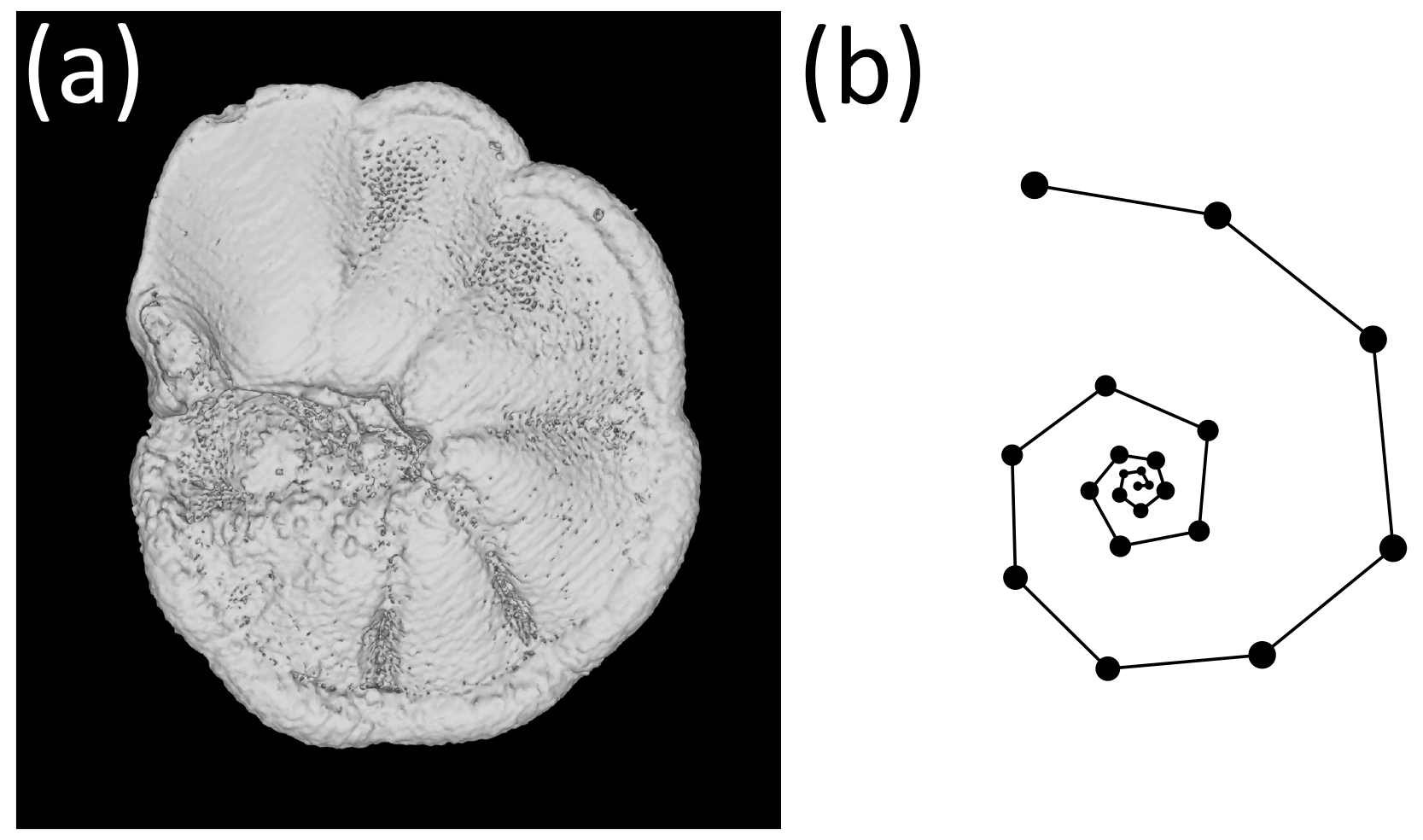
Figure 1 The exemplar Menardella limbata specimen released with the package. (a) CT scan of the exemplar M. limbata specimen. (b) Chamber centroids and growth spiral of the exemplar M. limbata specimen. Code to generate an interactive figure of (b) can be found in the code in the Supplement, lines 44–50.

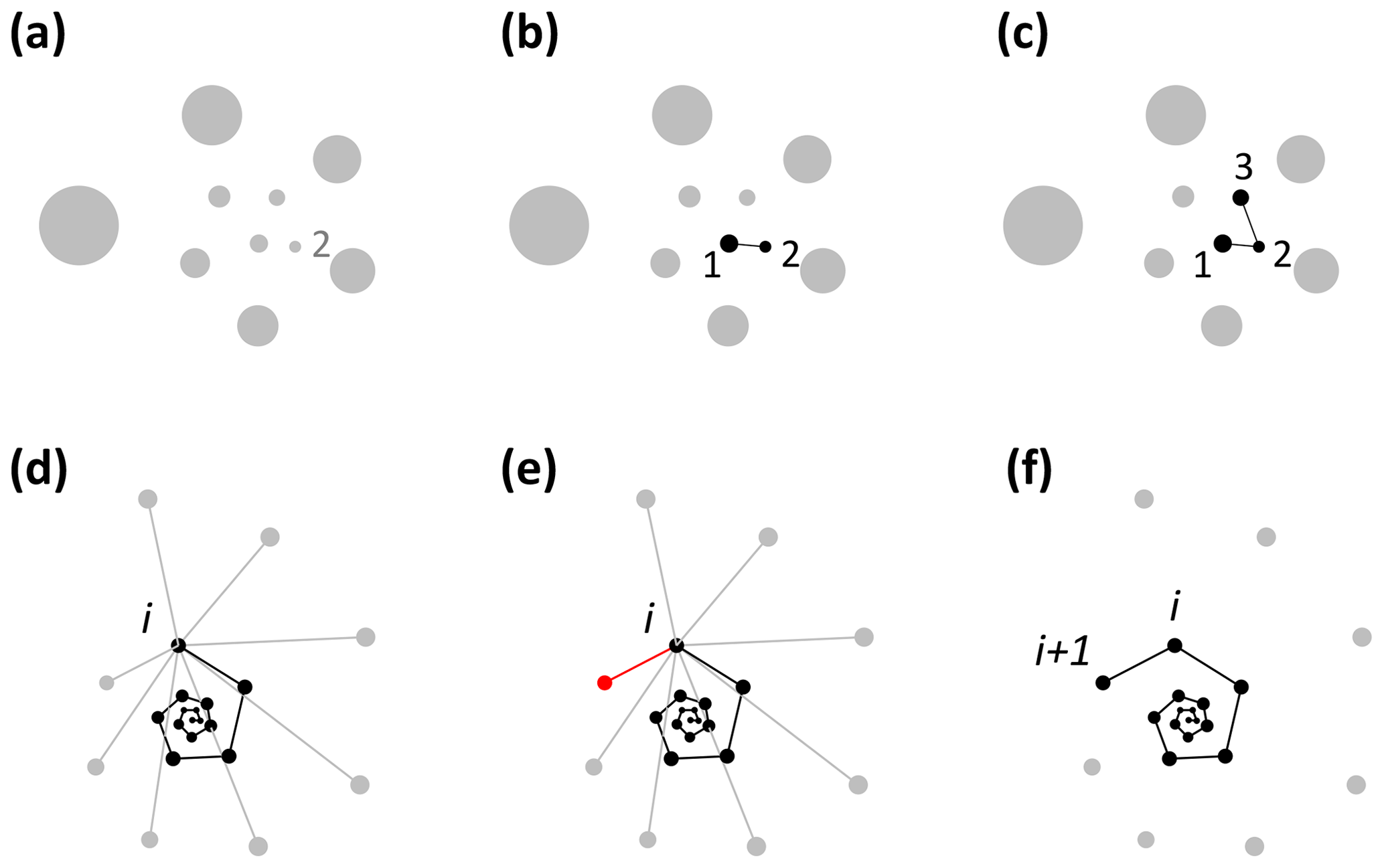
Figure 2 Visualisation of the chamber-ordering algorithm in the exemplar Menardella limbata data released with the package. (a–c) Discs represent chamber centroids of the earliest chambers, with disc size indicating chamber size. (a) The smallest chamber is chamber 2. (b) The closest chamber to chamber 2 is chamber 1. (c) The next closest chamber to chamber 2 is chamber 3. (d–f) Finding chamber i+1 when chambers 1 to i have been assigned. Black and grey dots represent centroids of ordered and unordered chambers, respectively. (d) Calculation of the distance from chamber i to all remaining chambers. (e) The closest unassigned chamber (red) to chamber i is chamber i+1 (f).

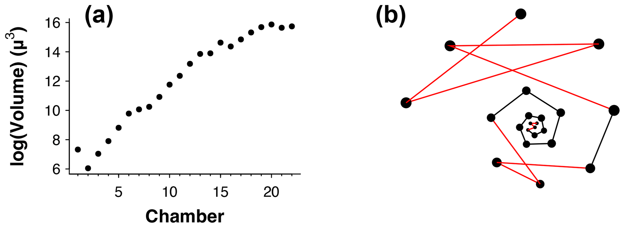
Figure 3 (a) Chamber size through ontogeny and (b) chambers ordered (incorrectly) by size only from the exemplar Menardella limbata data released with the package. The code in the Supplement, lines 67–80, can be used to generate an interactive plot of (b).

Occasionally, the proloculus is not present in fossil specimens, for example due to dissolution of the earliest chambers (Johnstone et al., 2010; Iwasaki et al., 2015). In that case, the algorithm takes the smallest chamber as the starting point. This version of the algorithm is less reliable than the version with the proloculus, as size does not always increase between subsequent chambers. For example, in Fig. 3a, if only chambers 15–22 were preserved, the algorithm would assign chamber 16 as the earliest chamber (rather than chamber 15). Generally, chamber size alone is not a reliable means to determine the order of growth. A number of species, such as the Menardella lineage, show reduced growth in the final chambers; small bullae on top of the final chamber are common, and occasionally unusually small chambers are found in random locations in the ontogeny (Duan et al., 2021). These deviations of the growth trajectory can have a profound effect on the resulting chamber order (Fig. 3b).

2.1.2 Usage

The function requires vectors with chamber x-, y- and z-centroid coordinates and chamber volume (code in the Supplement, lines 63–89). Its default version assumes that the proloculus is present but can be changed to proloculus=FALSE if necessary. It returns a data frame with the original data ordered by the newly assigned chamber numbers. See below for an example of the function usage in R. See Sect. A1 in Appendix A for function output.

with(Mlimbata, order.chambers(x=Cen
troidx, y=Centroidy, z=Centroidz,
V=Volume, proloculus=TRUE))

2.2 Checking the chamber order

Once chambers have been ordered (either by algorithm or manually), the R package contains a function that checks the chamber order and identifies unusual growth patterns to identify incorrectly ordered specimens. In foraminifera specimens with three or more chambers per whorl, the angle between subsequent chambers is ≥60^∘. Therefore, sequences with angles smaller than 60^∘ could be an indication of incorrectly ordered chambers. Common reasons for unusual sequences include manual error, faulty data or disrupted growth. The algorithm flags up any specimens that need additional inspection.

2.2.1 Algorithm: angles

Angles between subsequent chambers are calculated using the chamber.angles() function (code in the Supplement, lines 97–104). It requires vectors with chamber x-, y- and z-centroid coordinates and returns a vector with the angle every chamber makes with its previous two chambers (in degrees). Note that angles are generated from the third chamber onwards because the first and second chamber sit on a straight line.

2.2.2 Usage

The function requires vectors with chamber x-, y- and z-centroid coordinates. It returns a vector with the angle each chamber makes relative to the previous two previous chambers (see the code in the Supplement, lines 97–104). Note that at least three chambers are required for angle determination; therefore, no angles can be calculated for chambers 1 and 2. Code shown below is for the exemplar M. limbata specimen. See Fig. 5 and Sect. A2 for function output. See the code in the Supplement, line 104, for the output for T. sacculifer.

with(Mlimbata, chamber.angles(x=Cen
troidx, y=Centroidy, z=Centroidz))

2.2.3 Algorithm: chamber order check

To detect incorrectly ordered specimens, the algorithm calculates all angles α_i that chamber i makes with the previous two chambers i−1 and i−2 (Fig. 4). Angle α₃ is discarded if the proloculus is known to be present: the first three chambers form a triangle, and α₃ therefore forms an angle smaller than 60^∘ with the proloculus and deuteroconch. In specimens where the first few chambers are absent, for example due to dissolution, all chamber angles are considered. Specimens with all angles larger than 60^∘ are labelled as correctly ordered (Fig. 6a). Any specimens with one or more angles smaller than 60^∘ are flagged to the user as potentially incorrectly ordered specimens.

Figure 4 Chamber i is added at angle α_i relative to the previous two chambers.

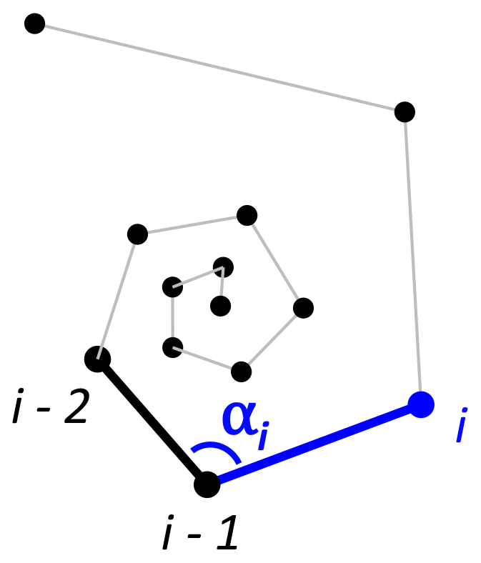
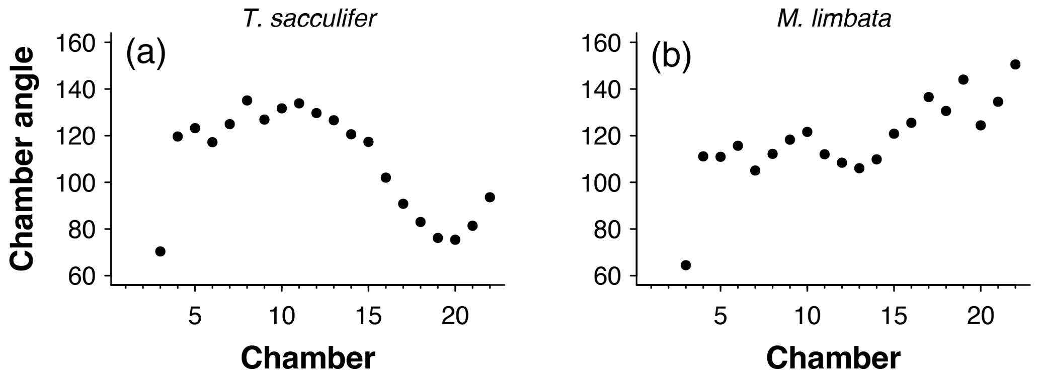
Figure 5 Angles between subsequent chambers for (a) Trilobatus sacculifer and (b) Menardella limbata.

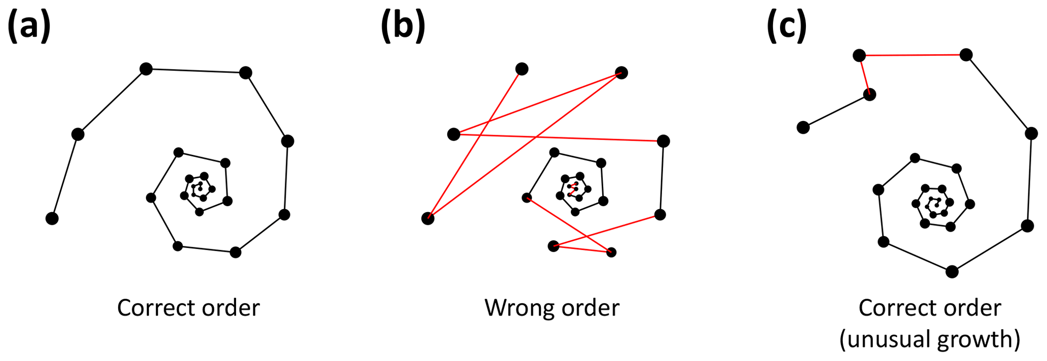
Figure 6 Three examples of correct and incorrect chamber sequences using the exemplar Menardella limbata data released with the package. Specimen (a) is a correctly ordered specimen with all angles larger than 60^∘. Specimen (b) is not ordered correctly and contains multiple angles much smaller than 60^∘ (red lines) as a result. Specimen (c) is correctly ordered but contains a sharp angle due to unusual growth of the penultimate chamber and is therefore flagged as an individual that needs closer inspection (note that the flagged angle appears larger than 60^∘ due to two-dimensional representation).

Specimens with angles smaller than 60^∘ either represent true negatives with one or more incorrectly ordered chambers (Fig. 6b) or specimens that experienced unusual growth resulting in sharp angles (Fig. 6c). Unusual growth can include a bulla or a smaller-than-expected chamber elsewhere in the sequence. Any manually ordered specimens flagged as incorrectly ordered can be run through the chamber-ordering algorithm to attempt to correct to sequence. If the sequence still returns sharp angles after ordering, the specimen needs to be inspected manually. In a preliminary analysis of 60 specimens, manual inspection was necessary for 5 % of the specimens. In all cases unusual growth was the cause of the ordering issues.

2.2.4 Usage

The function requires vectors with chamber x-, y- and z-centroid coordinates. The default option assumes that the proloculus is present, which can be changed to proloculus=FALSE if necessary. It returns a vector with either “correct order” if all angles are larger than 60^∘ or “check chamber order” if at least one chamber angle is smaller than 60^∘. See the code in the Supplement, lines 67 and 74, for examples. See Sect. A3 for function output.

with(Mlimbata, check.chamber.order(x=Cen
troidx, y=Centroidy, z=Centroidz,
proloculus=TRUE))

2.3 Number of chambers in the final whorl

The number of chambers in the final whorl is a frequently used diagnostic feature in taxonomy and can help distinguish between species and genera (e.g. Kennett and Srinivasan, 1983; Olsson et al., 1999; Pearson et al., 2006; Wade et al., 2018). Traditionally this number is determined from scanning electron microscope (SEM) or light microscope images and only describes the visible outer whorl. In contrast, CT scans also reveal all inner chambers. Using chamber centroid coordinates from CT data, we can determine the number of chambers in the final whorl at the time each chamber was built (Fig. 7). These new data could provide new insights into when ontogeny differences in whorl size between species and genera first arise. Manual determination of the number of chambers in the final whorl can be ambiguous, resulting in the inclusion of partial chambers in the final number (e.g. Globoconella inflata is described as having 3–3.5 chambers in the final whorl). These manual results are subjective and depend on visual volume determination of a partially hidden chamber. The function presented here uses distance between chambers to identify which chamber in the previous whorl is closest to the chamber under consideration. Therefore, the output is always in integers and no incomplete parts of chambers are considered.

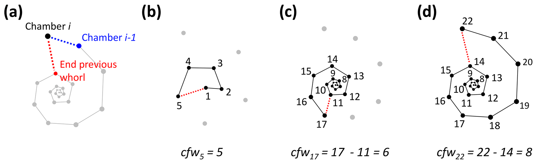
Figure 7 Determining the number of chambers in the final whorl for Menardella limbata at the time chamber i was built (cfw_i). (a) The two closest chambers to chamber i are chamber i−1 (blue) and the final chamber of the previous whorl (red). (b) If the closest non-neighbouring chamber is the proloculus, the chamber forms part of the first whorl and cfw_i=i. (c, d) If the closest chamber in the whorl below is not the proloculus, cfw_i=i − final chamber of previous whorl.

2.3.1 Algorithm

To calculate the number of chambers in the final whorl at the time chamber i was built (cfw_i), the algorithm searches for the closest chamber in the whorl immediately below chamber i. This chamber marks the end of the previous whorl (see Fig. 8a). Depending on the chamber configuration, the closest chamber to chamber i can be either chamber i−1 or the chamber in the whorl below. The algorithm selects the chamber with the shortest distance to chamber i that is not chamber i−1. If the closest non-neighbouring chamber to chamber i is chamber 1, chamber i is in the first and only whorl at time i (see Fig. 8b). In this case, cfw_i=i. If the final chamber of the previous whorl is not the proloculus, cfw${}_i=i-\mathit{\#}$ final chamber of previous whorl (Fig. 8c, d).

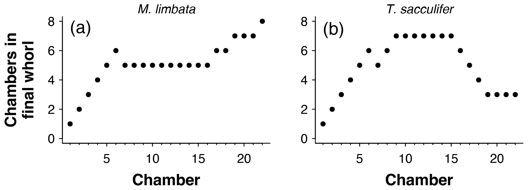
Figure 8 The number of chambers in the final whorl at the time each chamber was built using the exemplar (a) Menardella limbata and (b) Trilobatus sacculifer data.

2.3.2 Usage

The function requires vectors with chamber x-, y- and z-centroid coordinates. It returns a two-column data frame with the closest non-neighbouring chamber to each chamber and the number of chambers in the final whorl at the time each chamber was built (see the code in the Supplement, lines 115–122). Results shown are for the exemplar M. limbata specimen. See Sect. A4 for function output. See the code in the Supplement, line 122 for the output for T. sacculifer.

with(Mlimbata, chambers.in.whorl(x=Cen
troidx, y=Centroidy, z=Centroidz))

2.4 Number of whorls

Taxonomic descriptions often include the number of whorls typically found in adult specimens (e.g. Kennett and Srinivasan, 1983; Olsson et al., 1999; Pearson et al., 2006; Wade et al., 2018). Three to four whorls are common in planktonic foraminifera, whereas benthic foraminifera, especially larger species, can have many more (Holbourn et al., 2013). Differences in the numbers of whorls among specimens can help species identification. A change in the number of whorls through time can point to an altered developmental history, such as paedomorphosis (reduced development) or peramorphosis (extended development).

To determine the total number of whorls, all chambers need to be visible. Determining the number of whorls manually can introduce bias similar to counting the number of chambers in the final whorl by eye. By letting an algorithm find the closest chamber in the whorl below individual chambers from CT scan data, the number of whorls can be determined objectively.

2.4.1 Algorithm description

The algorithm starts with the proloculus and makes its way up the logarithmic spire from there. The first whorl consists of all chambers whose closest non-neighbouring chamber is the proloculus (Fig. 9a). The second whorl starts with the first chamber whose closest chamber in the whorl below is not the proloculus (chamber 7 in Fig. 9a). Subsequently, whorl i+1 starts with the first chamber whose closest chamber in the whorl below is in whorl i (Fig. 9b). The last whorl is often not complete (e.g. Pearson et al., 2006) (Fig. 9c). The algorithm checks if the last whorl is complete by comparing the number of chambers in the last whorl as determined algorithmically (counted forward from the proloculus onwards) with the number of chambers in the final whorl at the time the final chamber was built (counted backwards, starting with the final chamber). If these numbers are not the same, all chambers in the last whorl are flagged as being part of an incomplete whorl. For example, the specimen in Fig. 9c had eight chambers in its final whorl at the time the final chamber was built, but only five of these were part of the actual last whorl.

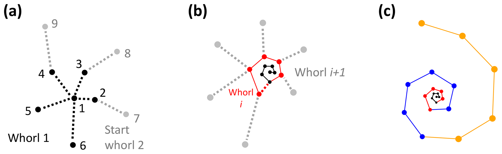
Figure 9 Determining the total number of whorls for the example Menardella limbata specimen. (a) The first whorl consists of all chambers whose closest chamber is the proloculus (black). Whorl 2 (grey) starts with the first chamber whose closest neighbour in the whorl below is not the proloculus. (b) Whorl i+1 (grey) starts with the first chamber that has a chamber from whorl i (red) as its closest non-neighbouring chamber. (c) All three complete whorls (black, red, blue) and the fourth incomplete whorl (orange).

2.4.2 Usage

The function requires vectors with chamber x-, y- and z-centroid coordinates. It returns a two-column data frame with the whorl number of each chamber and whether the whorl is complete (code in the Supplement, lines 124–130). All whorls but the final whorl are complete by definition, whereas the final whorl is either complete or incomplete. See Sect. A5 for function output.

with(Mlimbata, whorl(x=Cen
troidx, y=Centroidy, z=Centroidz))

2.5 Coiling direction

Coiling direction is an important trait for biostratigraphy, with changes in the dominant coiling direction marking biostratigraphic horizons (e.g. Wade et al., 2011). For some species the coiling direction is the primary means of identification, such as in Neogloboquadrina pachyderma and N. incompta (Darling et al., 2006). Although the coiling direction of adult individuals can easily be determined by eye, the coiling of earlier, hidden ontogenetic stages is more difficult to analyse. The R package includes a function that determines the coiling direction throughout ontogeny. This could prove useful to determine the exact moment of coiling change in the rare planktonic foraminifera species that build whorl-enveloping chambers such as Orbulinoides beckmanni or more likely in streptospirally coiled benthic foraminifera species.

2.5.1 Algorithm

To determine the coiling direction of chamber i we compare the vertical direction of growth to the cross product of the vectors v and w between chambers i−2, i−1 and i. The cross product creates a vector perpendicular to both v and w, with the direction of v×w determined by the direction of travel from v to w (Fig. 10). Clockwise travel as viewed from the umbilical side (i.e. sinistral coiling) produces a cross-product vector pointing away from the vertical direction of growth, whereas anticlockwise travel as viewed from the umbilical side (i.e. dextral coiling) produces a vector pointing in the same direction as the direction of vertical growth (give or take minor deviations). Therefore, if the angle between v×w and the direction of growth is smaller than 90^∘, the coiling direction is anticlockwise or dextral, whereas an angle larger than 90^∘ indicates clockwise or sinistral coiling.

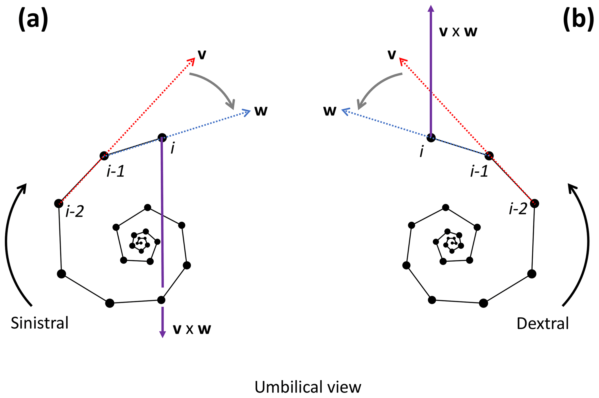
Figure 10 Determination of the coiling direction of chamber i for the example Menardella limbata specimen. (a) If the direction of change from vector v through chambers i−2 and i−1 (red) and vector w through chambers i−1 and i (blue) is clockwise as viewed from the umbilical side (i.e. sinistral coiling), the cross-product v×w (purple) points towards the proloculus in the opposite direction to the direction of growth. (b) If the direction of change from v to w is anticlockwise as viewed from the umbilical side (i.e. dextral coiling) v×w aligns with the direction of growth. Note that the orientation of the specimen does not influence the coiling direction outcome of the algorithm: if the same specimens were viewed from the spiral side, both the cross product and the direction of growth would flip by 180^∘, maintaining their similar or opposite relationship necessary to determine the coiling direction.

2.5.2 Usage

The function requires vectors with chamber x-, y- and z-centroid coordinates. It returns a vector with the coiling direction of each chamber relative to the two previous chambers (see the code in the Supplement, lines 132–138). Note that at least three chambers are required for coiling direction determination; therefore, no coiling direction can be established for chambers 1 and 2. Also note that the earliest chambers in the juvenile stage grow nearly planispirally, the smallest deviations from which can result in an apparent change of coiling direction. See Sect. A6 for function output.

with(Mlimbata, coiling.direction(x=Cen
troidx, y=Centroidy, z=Centroidz))

2.6 Trochospirality

The height of the trochospire is another trait used to distinguish among species (Fabbrini et al., 2021; Biolzi, 1991) and genera (Gradstein and Waskowska, 2021; Lipps, 1966; Pearson and Coxall, 2014). Specimens are qualitatively described as either planispiral (Fig. 11a) or having a low or high trochospire (Fig. 11b, c), but there is currently no direct way to quantify the height or angle of the trochospire. Quantifying the trochospire can help determine the exact moment of evolutionary divergence of two closely related species through statistical analyses (e.g. Pearson and Ezard, 2014). The height of the trochospire has also been noted to change through ontogeny: growth is nearly planispiral in the juvenile stage but increases as individuals mature (Caromel et al., 2016; Apthorpe, 2020; Kendall et al., 2020; Poole and Wade, 2019; Morard et al., 2019). The timing of change could be used to determine the transition from the juvenile to the neanic stage, which is currently only described qualitatively through manual inspection (Brummer et al., 1986, 1987).

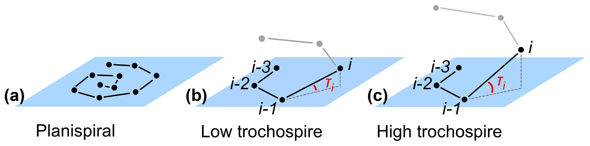
Figure 11 Theoretical examples of (a) planispiral growth and (b, c) low and high trochospires, respectively. Planes represent the growth plane of the entire specimen in the case of planispiral growth (a) or the plane defined by chambers i−3, i−2 and i−1 for non-planispiral growth (b, c); τ_i is the trochospire angle of chamber i relative to the plane defined by the previous three chambers.

2.6.1 Algorithm

Shells growing in approximate logarithmic spirals, such as ammonoids and gastropods, are traditionally described using “Raupian” parameters (Raup, 1966, 1967) that quantify growth relative to the coiling axis. The translation rate or growth in the direction of the coiling axis for every ontogenetic step can theoretically be used to calculate trochospirality in foraminifera (Morard et al., 2019; Caromel et al., 2016). This method depends on correct identification of the coiling axis. Ammonoids and gastropods grow continuously and roughly isometrically, making the coiling axis easy to identify. Foraminifera, however, grow in discrete steps, and growth patterns change through ontogeny (Signes et al., 1993). Therefore, the coiling axis of a foraminifera specimen changes through ontogeny and is impossible to determine mathematically. Approximations of the coiling axis would need to be done by hand, potentially introducing bias and influencing any resulting calculations of trochospirality.

Alternatively, we can define the trochospirality of chamber i as the angle between chamber i and the plane defined by the previous three chambers (Fig. 11). This method does not rely on a coiling axis and only requires chamber centroid coordinates. Specimens following a perfect logarithmic spiral will have a constant trochospirality value throughout ontogeny. However, natural growth is rarely perfect. The trochospirality of a specimen can be defined as the average trochospirality τ_i of all chambers, and deviations in τ_i can be used to assess developmental plasticity and ontogenetic constraints (Fig. 12).

2.6.2 Usage

The function requires vectors with chamber x-, y- and z-centroid coordinates. It returns a vector with the trochospirality angle of each chamber, relative to the plane formed by the previous three chambers (see the code in the Supplement, lines 106–113). Note that at least three previous chambers are required to form a plane. Therefore, no trochospirality angle exists for the first three chambers. See Sect. A7 for function output.

with(Mlimbata, trochospirality(x=Cen
troidx, y=Centroidy, z=Centroidz))

3 Package applications and future work

For ease of use, all trait functions have been combined into a single function: foram.growth.3D(). This function requires vectors with chamber number, centroid coordinates and volumes and returns a data frame with the original data, plus angles between subsequent chambers, trochospirality, chambers in the final whorl at the time each chamber was built, the whorl number each chamber belongs to, whether the whorl is complete, coiling direction, and chamber order (see the code in the Supplement, lines 140–150). See Sect. A8 for function output.

with(Mlimbata, foram.growth.3D(n=Cham
ber, x=Centroidx, y=Centroidy,
z=Centroidz, proloculus=TRUE))

Figure 12 Trochospirality per chamber for the exemplar data of (a) Trilobatus sacculifer and (b) Menardella limbata.

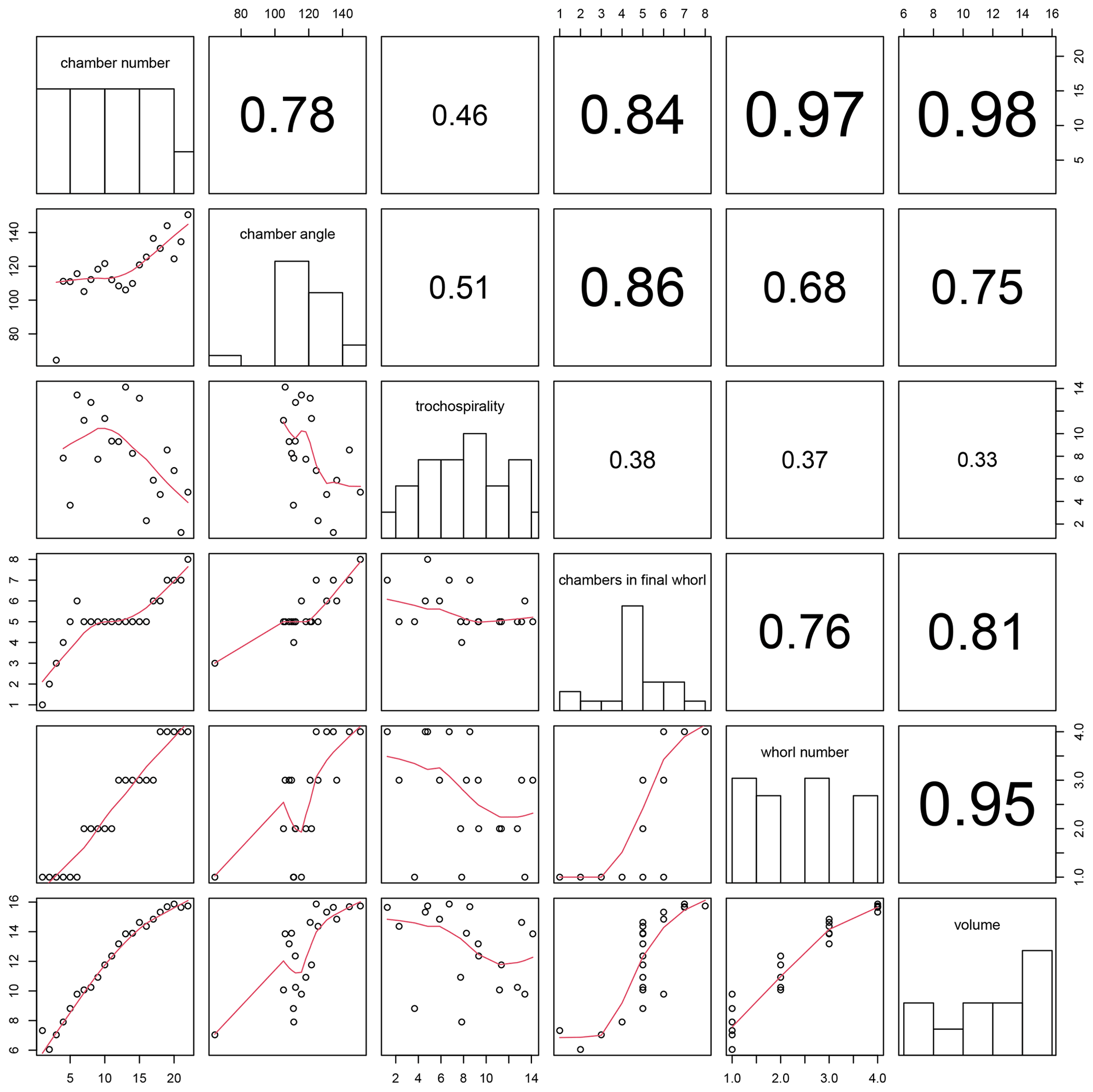
Figure 13 Correlation between all combinations of traits calculated for the example Menardella limbata specimen by the foram3D package. Plots on the diagonal show histograms of the trait data. Plots below the diagonal show all combinations of traits plotted against each other, with red lines representing splines. R² values of all trait correlations are shown in the panels above the diagonal. The column on the far left shows all trait values through ontogeny. The next column shows all remaining traits plotted against chamber angle.

Plotting combinations of traits against each other can reveal ontogenetic trajectories and trait covariation patterns through ontogeny. The example data show stable chamber angles until around chamber 14, when angles increase with chamber number (Fig. 13, far left column). Trochospirality and growth rate decrease around the same time, with the number of chambers in the final whorl increasing several chambers later. The remaining columns in Fig. 13 show the correlations between all remaining trait combinations. Strong covariations between some traits are expected, such as whorl number and chamber volume (Fig. 13, bottom row, second from right), because chambers in earlier whorls are typically smaller. Others, such as the covariation between the number of chambers in the final whorl and chamber volume (Fig. 13, bottom row, third from right), are not immediately obvious and could point to a size threshold for whorl expansion. Similarly, chamber angles increase at the same time the rate of chamber growth starts to decrease, several chambers before the number of chambers in the final whorl increases, suggesting a switch away from isometric growth that leads to a reduced chamber-by-chamber growth rate and thus increasing numbers of chambers in the final whorl.

4 Prospects for future work

We present a new R package to automatically reconstruct foraminifera growth trajectories from chamber x, y and z centroid coordinates. The package functions arrange chambers in order of growth, calculate distances and angles between chambers, determine the total number of whorls and the number of chambers in the final whorl at the time each chamber was built, and, for the first time, quantify trochospirality. Applied to large numbers of specimens through multiple lineages and evolutionary transitions, the foram3D package functions can shed new light on ontogenetic trajectories and developmental constraints through time. They can be used to quantify ontogenetic stages, for example through changes in trochospirality in the juvenile and neanic stages or the increase in chambers in the final whorl for the neanic to adult transition. Additionally, they can be used to quantify species differences, for example through average trochospirality, angles between chambers in the final whorl and the total number of whorls. This will be particularly valuable for determining the exact moment of the origination of a new species, which is often difficult to identify by eye. Our package enables multivariate analyses of the incredible richness from x-ray CT data and could substantially improve our understanding of developmental constraints on planktonic foraminifera growth and form.

Appendix A

“NA” stands for “not available” and indicates an empty entry.

A1 Output of the function that orders chambers in the direction of growth

with(Mlimbata, order.chambers(x=Centroidx, y=Centroidy, z=Centroidz, V=Volume,
proloculus=TRUE))

##	x centroid	y centroid	z centroid	Volume	Chamber number
## 1	790.2737	947.1173	453.7312	1519.0677	1
## 2	800.3547	954.0144	450.9993	423.1689	2
## 3	801.7997	944.2201	464.2364	1139.3008	3
## 4	785.5543	936.5239	468.6528	2707.1956	4
## 5	770.2097	941.8412	454.1172	6727.2998	5
## 6	779.0149	952.0797	431.4037	17740.5406	6
## 7	810.6712	947.0431	431.7093	23588.9512	7
## 8	819.5385	925.7222	454.7856	28146.1542	8
## 9	792.6812	907.2282	473.0768	55277.7883	9
## 10	748.8339	906.8281	458.0008	127824.1210	10
## 11	743.5526	931.0394	400.9859	233106.3626	11
## 12	815.3179	941.4148	371.8330	530149.1992	12
## 13	876.3621	888.9579	429.9081	1040610.1960	13
## 14	818.6441	827.8897	498.2896	1085341.3140	14
## 15	710.8669	810.0553	481.1860	2250536.7620	15
## 16	651.7275	847.0710	393.0151	1730125.8720	16
## 17	675.3247	899.9679	290.0133	2798247.4690	17
## 18	798.6004	930.2500	228.4772	4510008.8980	18
## 19	949.4519	901.2303	231.3315	6496217.0310	19
## 20	1036.1169	801.7007	365.4462	7777235.9650	20
## 21	982.8341	716.6077	509.5566	6215726.6070	21
## 22	863.8481	657.6218	603.0626	6834399.4760	22

A2 Output of the function calculating angles between subsequent chambers

with(Mlimbata, chamber.angles(x=Centroidx, y=Centroidy, z=Centroidz))

## [1]	NA	NA	64.47616	111.14269	110.93628	115.67051	105.06948
## [8]	112.18464	118.27829	121.63305	112.03424	108.40934	106.04217	109.85145
## [15]	120.83569	125.51267	136.54085	130.60246	144.03099	124.42830	134.53817
## [22]	150.52445

A3 Output of the function checking the chamber order

with(Mlimbata, check.chamber.order(x=Centroidx, y=Centroidy, z=Centroidz,
proloculus=TRUE))

## [1]	"Correct"	"Correct"	"Correct"	"Correct"	"Correct"	"Correct"	"Correct"
## [8]	"Correct"	"Correct"	"Correct"	"Correct"	"Correct"	"Correct"	"Correct"
## [15]	"Correct"	"Correct"	"Correct"	"Correct"	"Correct"	"Correct"	"Correct"
## [22]	"Correct"

A4 Output of the function determining the number of chambers in the final whorl at the time chamber i was built

with(Mlimbata, chambers.in.whorl(x=Centroidx, y=Centroidy, z=Centroidz))

##	Closest chamber	Chambers in whorl
## [1,]	1	1
## [2,]	1	2
## [3,]	1	3
## [4,]	1	4
## [5,]	1	5
## [6,]	1	6
## [7,]	2	5
## [8,]	3	5
## [9,]	4	5
## [10,]	5	5
## [11,]	6	5
## [12,]	7	5
## [13,]	8	5
## [14,]	9	5
## [15,]	10	5
## [16,]	11	5
## [17,]	11	6
## [18,]	12	6
## [19,]	12	7
## [20,]	13	7
## [21,]	14	7
## [22,]	14	8

A5 Output of the function determining which whorl each chamber belongs to

with(Mlimbata, whorl(x=Centroidx, y=Centroidy, z=Centroidz))

##	Whorl number	Whorl complete?
## 1	1	complete
## 2	1	complete
## 3	1	complete
## 4	1	complete
## 5	1	complete
## 6	1	complete
## 7	2	complete
## 8	2	complete
## 9	2	complete
## 10	2	complete
## 11	2	complete
## 12	3	complete
## 13	3	complete
## 14	3	complete
## 15	3	complete
## 16	3	complete
## 17	3	complete
## 18	4	incomplete
## 19	4	incomplete
## 20	4	incomplete
## 21	4	incomplete
## 22	4	incomplete

A6 Output of the function determining coiling direction at the time chamber i was built

with(Mlimbata, coiling.direction(x=Centroidx, y=Centroidy, z=Centroidz))

## [1]	NA	NA	"sinistral"	"sinistral"	"sinistral"	"dextral"
## [7]	"dextral"	"dextral"	"dextral"	"dextral"	"dextral"	"dextral"
## [13]	"dextral"	"dextral"	"dextral"	"dextral"	"dextral"	"dextral"
## [19]	"dextral"	"dextral"	"dextral"	"dextral"

A7 Output of the function calculating trochospirality

with(Mlimbata, trochospirality(x=Centroidx, y=Centroidy, z=Centroidz))

## [1]	NA	NA	NA	7.835840	3.664881	13.421233	11.177728
## [8]	12.761478	7.737775	11.345215	9.337931	9.295332	14.123845	8.254441
## [15]	13.135575	2.295534	5.876539	4.614813	8.554413	6.731464	1.251507
## [22]	4.820587

A8 Output of the function combining the outputs of all functions described above

with(Mlimbata, foram.growth.3D(n=Chamber, x=Centroidx, y=Centroidy, z=Centroidz,
proloculus=TRUE))

##	Chamber number	Centroid x	Centroid y	Centroid z	Chamber angle
## 1	1	790.2737	947.1173	453.7312	NA
## 2	2	800.3547	954.0144	450.9993	NA
## 3	3	801.7997	944.2201	464.2364	64.47616
## 4	4	785.5543	936.5239	468.6528	111.14269
## 5	5	770.2097	941.8412	454.1172	110.93628
## 6	6	779.0149	952.0797	431.4037	115.67051

##	Trochospirality	Chambers in final whorl	Whorl number	Whorl complete?
## 1	NA	1	1	complete
## 2	NA	2	1	complete
## 3	NA	3	1	complete
## 4	7.835840	4	1	complete
## 5	3.664881	5	1	complete
## 6	13.421233	6	1	complete

##	coiling direction	chamber order
## 1	〈NA〉	Correct
## 2	〈NA〉	Correct
## 3	sinistral	Correct
## 4	sinistral	Correct
## 5	sinistral	Correct
## 6	dextral	Correct