Artificial intelligence applied to the classification of eight middle Eocene species of the genus Podocyrtis (polycystine radiolaria)

This study evaluates the application of artificial intelligence (AI) to the automatic classification of radiolarians and uses as an example eight distinct morphospecies of the Eocene radiolarian genus Podocyrtis, which are part of three different evolutionary lineages and are useful in biostratigraphy. The samples used in this study were recovered from the equatorial Atlantic (ODP Leg 207) and were supplemented with some samples coming from the North Atlantic and Indian Oceans. To create an automatic classification tool, numerous images of the investigated species were needed to train a MobileNet convolutional neural network entirely coded in Python. Three different datasets were obtained. The first one consists of a mixture of broken and complete specimens, some of which sometimes appear blurry. The second and third datasets were leveled down into two further steps, which excludes broken and blurry specimens while increasing the quality. The convolutional neural network randomly selected 85 % of all specimens for training, while the remaining 15 % were used for validation. The MobileNet architecture had an overall accuracy of about 91 % for all datasets. Three predicational models were thereafter created, which had been trained on each dataset and worked well for classification of Podocyrtis coming from the Indian Ocean (Madingley Rise, ODP Leg 115, Hole 711A) and the western North Atlantic Ocean (New Jersey slope, DSDP Leg 95, Hole 612 and Blake Nose, ODP Leg 171B, Hole 1051A). These samples also provided clearer images since they were mounted with Canada balsam rather than Norland epoxy. In spite of some morphological differences encountered in different parts of the world's oceans and differences in image quality, most species could be correctly classified or at least classified with a neighboring species along a lineage. Classification improved slightly for some species by cropping and/or removing background particles of images which did not segment properly in the image processing. However, depending on cropping or background removal, the best result came from the predictive model trained on the normal stacked dataset consisting of a mixture of broken and complete specimens.

1 Introduction

Polycystine radiolarians belong to an extant group of marine zooplankton protists secreting an aesthetically pleasing siliceous test that is rather well preserved in the fossil record and is therefore of importance to both biostratigraphy and paleoceanography. They are unique amongst skeleton-bearing planktonic representatives in having a fossil record stretching as far back as the early Cambrian (Obut and Iwata, 2000; Pouille et al., 2011; Aitchison et al., 2017). Their continuous Cenozoic fossil record has allowed description of a number of well-documented evolutionary lineages (Sanfilippo and Riedel, 1990), although their taxonomy has still not been fully clarified in spite of the great progress achieved during the last few decades (O'Dogherty et al., 2021). Polycystine radiolarian classification at the species level is based on morphological criteria, which therefore bear particular significance if one wishes to address evolutionary questions, but also for the development of high-resolution biostratigraphy.

Supervised learning uses labeled data to train algorithms that will enable automatic classification and computer vision to deal with information from a visual context such as digital images or videos. These are some of the branches of artificial intelligence (AI) that have been developed during the last few years and may provide solutions to a number of difficult classification tasks. As such, convolutional neural networks (CNNs) use a deep learning algorithm to recognize patterns in images in a grid-like arrangement with multiple layers (Hijazi et al., 2015), which is a common approach for the analysis and classification of images. Training CNNs in a supervised way requires both a labeled training and validation dataset, from which the CNNs will learn features and patterns unique to each class from the training set by forming outputs, with which the untrained validation data will respond to if the model is a good fit.

A number of studies have attempted to apply automatic classification techniques on microfossils and/or microremains by using supervised machine learning in the past. Dollfus and Beaufort (1999) were the first micropaleontologists to apply AI in classifying and counting coccolithophores. They created the software SYRACO as an automatic recognition system of coccoliths, which was further developed a few years later (Beaufort and Dollfus, 2004) to count automatically identified coccoliths but also for application to late Pleistocene reconstructions of oceanic primary productivity (Beaufort et al., 2001). Goncalves et al. (2016) tried to automatically classify modern pollen from the Brazilian savannah using different algorithms and achieved a highest median accuracy of 66 %, which is nearly as high as the median accuracy obtained by humans, based on a dataset that consisted of 805 specimens and 23 classes of pollen types. Hsiang et al. (2019) trained a neural network of 34 different modern species of foraminifera using a large dataset of a few thousand images, which reached an accuracy exceeding 87.4 %. Carvalho et al. (2020) used 3D images of 14 species of foraminifera, obtaining a dataset as large as 4600 specimens and a microfossil identification and segmentation accuracy as high as 98 % by using the CNN architectures of Resnet34 and Resnet50 with adjustment of hyperparameter optimization. De Lima et al. (2020) used a relatively small dataset of fusulinids composed of 342 images (including training, validation and test sets), which were divided into eight classes on a genus level to train in different CNNs architectures. They obtained the highest accuracy of 89 % by using the fine-tuning InceptionV3 model. Marchant et al. (2020) managed to train a CNN on a very large dataset of 13 001 images, including 35 different species of foraminifera. The best accuracy they obtained was about 90 %. Tetard et al. (2020) developed an automated method for new slide preparations, image capturing, acquisition and identification of radiolarians with the help of a software known as ParticleTrieur. They attempted to classify all common radiolarians existing since the Miocene, in a total of 132 classes, with 100 of them being relatively common species. They obtained an overall accuracy of about 90 %. Itaki et al. (2020) developed an automatization for the acquisition and deep learning of a single radiolarian species, Cycladophora davisiana, and obtained an accuracy similar to a human expert. Interestingly, they managed to be three times faster than a human being. Finally, Renaudie et al. (2018) applied the computationally efficient MobileNet convolutional neural network architecture for automatic radiolarian classification of 16 closely related species of the Cenozoic genera Antarctissa and Cycladophora. They obtained an overall accuracy of about 73 %, which they managed to increase to ca. 90 % after ignoring specimens which were not classified at all and by only including those specimens which had been given a class by the CNN.

The objective of our study was to obtain an accurate system of automatic classification for an automated classification of eight closely related species belonging to the middle Eocene genus Podocyrtis Ehrenberg, 1846 to be used by non-specialists in radiolarian taxonomy (e.g., students, industrial biostratigraphers or geochemists). Several of these species have a very good fossil record and are important in biostratigraphy as well as in morphometrics and evolutionary studies including gradual evolutionary transitions (Sanfilippo and Riedel, 1990; Danelian and MacLeod, 2019). In this work, we wished to implement MobileNet version 1 (Howard et al., 2017) because of its simplicity and lightweight construction, which enabled us to run more data in a shorter time. Many examples of MobileNet are available online and it is relatively easy to reproduce this work, which could thus be seen as a starting point for any other type of CNN implementation.

We will therefore attempt to answer the following scientific questions:

1. How well can the MobileNet convolutional neural network classify closely related species of the genus Podocyrtis?

2. How well can the predictive model classify Podocyrtis species under different processing settings and with materials coming from different parts of the world's ocean?

2 Materials

The main radiolarian material used for this study comes from the South American margin off Surinam (Demerara Rise, Ocean Drilling Program (ODP) Leg 207, Shipboard Scientific Party, 2004, see Table 1), where the middle Eocene interval is composed of an expanded sequence of chalk rich in abundant and well-preserved siliceous microfossils (for more details see Danelian et al., 2005, 2007; Renaudie et al., 2010). We focused on eight closely related species of the genus Podocyrtis (Fig. 1). Taxonomic concepts followed in this study are in accordance with Riedel and Sanfilippo (1970), Sanfilippo et al. (1985), Sanfilippo and Riedel (1990, 1992), with their stratigraphic ranges as specified recently by Meunier and Danelian (2022).

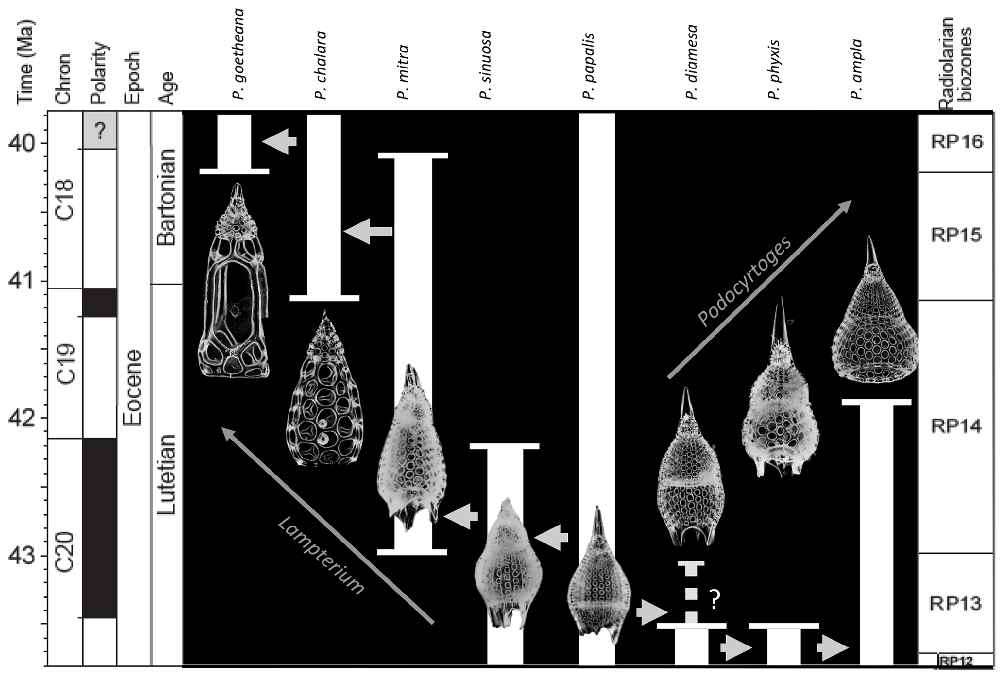
Figure 1 Age range and evolutionary relationships of Podocyrtis species occurring in Hole 1260A modified from Meunier and Danelian (2022). Arrows indicate descending species.

The eight studied species are considered to be part of three distinct evolutionary lineages, classified as three subgenera of the genus Podocyrtis: Podocyrtis, Podocyrtoges and Lampterium (Sanfilippo and Riedel, 1992). All taxonomic assignments were performed by a single taxonomist but were also checked by two other experts who had access to all 2D images of the dataset. The Podocyrtis species are in general relatively easy to recognize by their outer shape and/or size and distribution of pores (Figs. 1 and 2).

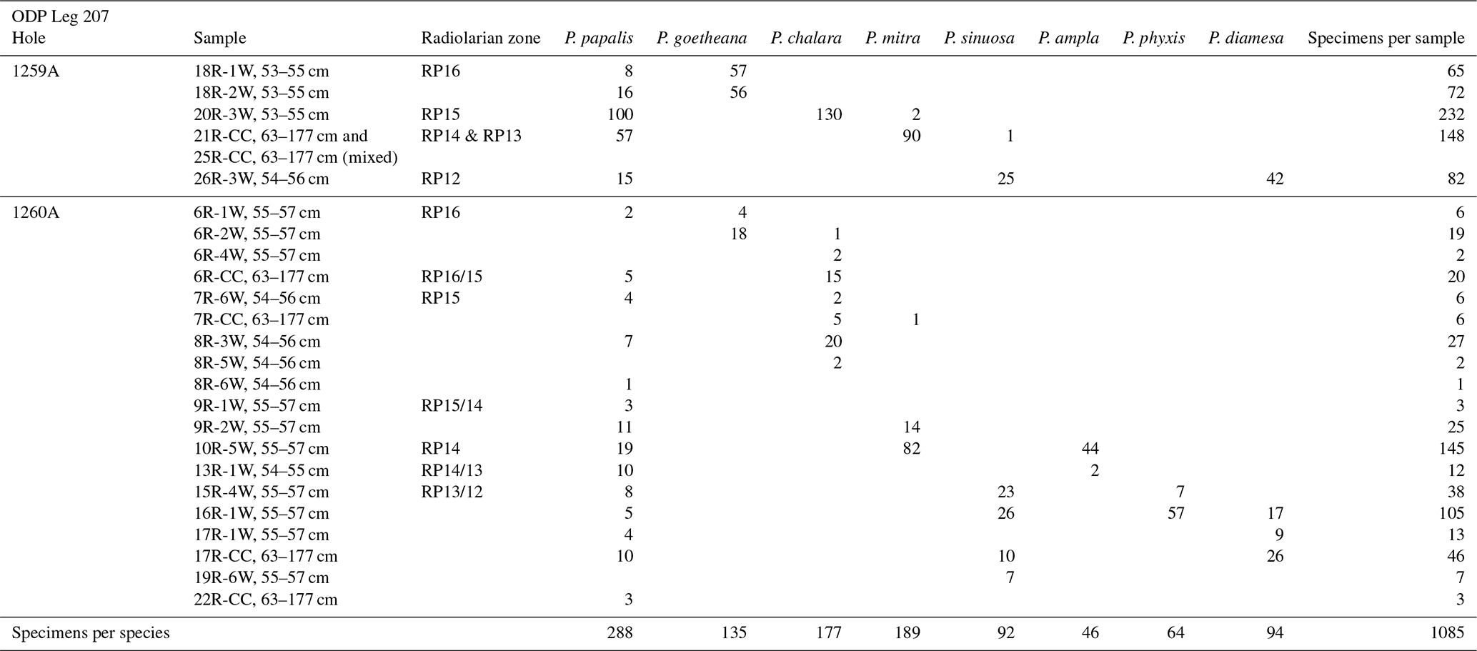
Table 1 Number of specimens per species for each sample coming from ODP Leg 207 which were used for training and validation.

The Podocyrtis subgenus represents an ancestral lineage that experienced morphological stasis. It is represented by the single morphospecies Podocyrtis papalis Ehrenberg, 1847, which differs from all the other Podocyrtis species by its partly developed abdomen (often smaller than the thorax), its overall fusiform shape (largest test width located on its thorax) and weakly expressed lumbar stricture. Three shovel shaped feet are often present, as well as a well-developed apical horn (which may be broken sometimes).

The Podocyrtoges subgenus is composed of three distinct morphospecies that belong to a lineage that evolved anagenetically. These are, from oldest to youngest:

Podocyrtis diamesa Riedel and Sanfilippo, 1970 differs from P. papalis by a more distinct lumbar stricture, with rather equally sized thorax and abdomen, and a more elongated than fusiform body. Some of the stratigraphically late forms of P. papalis display a degree of similarity in shape to P. diamesa (Fig. 2, 13th image), although the latter is much bigger in size (Fig. 1) and bears a larger apical horn than P. papalis.

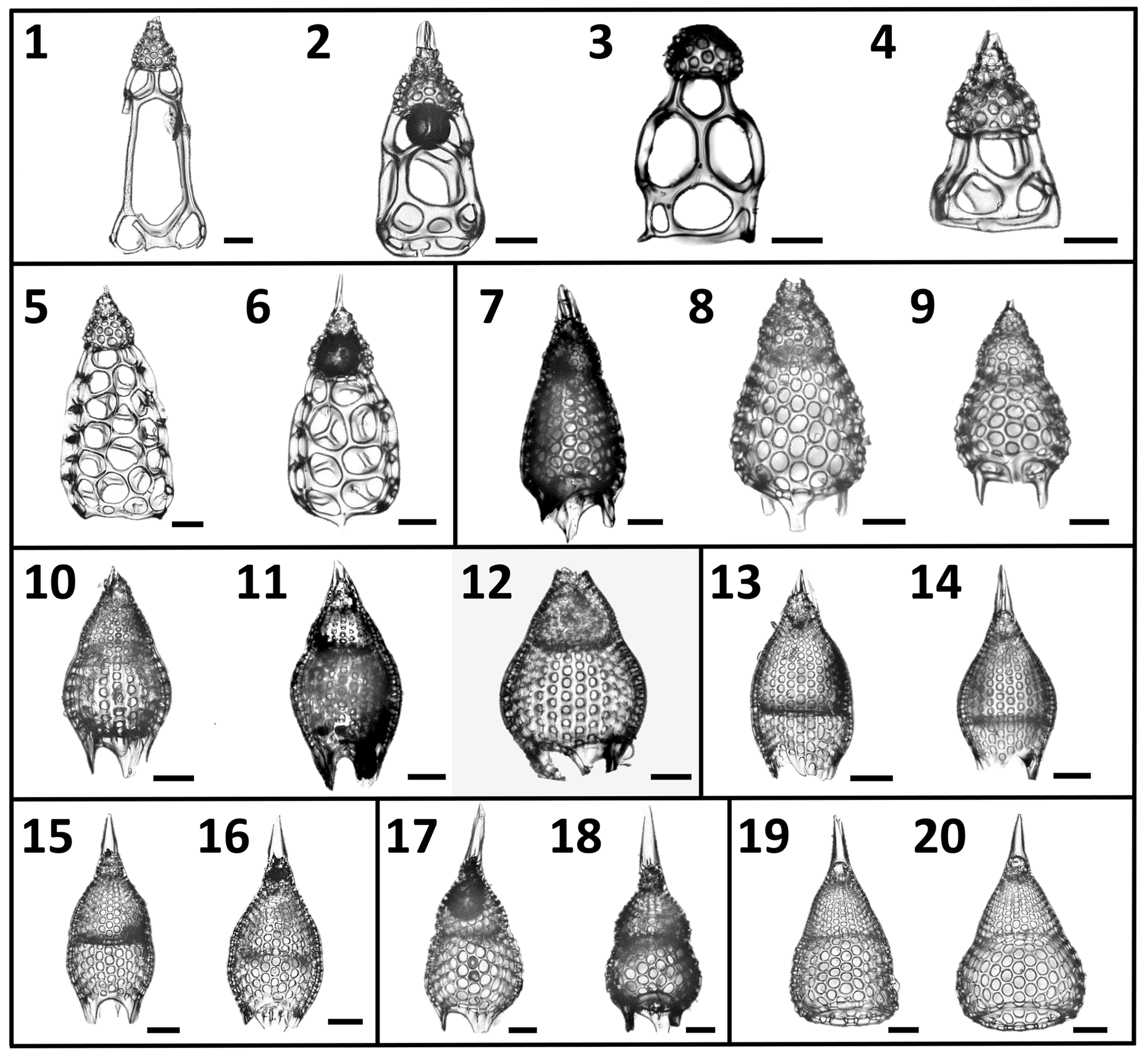
Figure 2 A selection of the variety of Podocyrtis morphotypes analyzed in this study. (1–4) P. goetheana. (1–2) from 207_ 1259A_ 18R_1W. 53–55 cm; (3) 207_1260A_6R_2W. 55–57 cm; (4) 207_ 1259A_ 18R_2W. 53–55 cm. (5–6) P. chalara from 207_1259A_20R_3W. 53–55 cm. (7–9) P. mitra from 207_1260A_10R_5W. 55–57 cm. (10–12) P. sinuosa. (10) from 207_1259A_26R_3W. 54–56 cm; (11) 207_1260A_19R_6W. 55–57 cm; (12) Indian Ocean. 115_711A _25X_1. 83–86 cm. (13–14) P. papalis. late (13) and typical (14) forms from 207_1259A_20R_3W. 53–55 cm. (15–16) P. diamesa from 207_1259A_ 26R_3W. 54–56 cm. (17–18) P. phyxis from 207_ 1260A_16R_1W. 55–57 cm. (19–20) P. ampla from 207_1260A_10R_5W. 55–57 cm. Scale bar is 50 µm.

Podocyrtis phyxis Sanfilippo and Riedel, 1973 displays a very distinct lumbar stricture formed at the junction between the abdomen and the thorax, with the former being more inflated than the latter. The overall outline of the test recalls the number eight “8”. In general, a large horn is present on the cephalis. Complete specimens were rare in our material, as their horn is fragile and often broken.

Podocyrtis ampla Ehrenberg, 1874 displays a conical outline and a less prominent lumbar stricture than P. phyxis, with its abdomen being widest distally. Stratigraphically late forms of P. ampla do not display any feet and these forms were selected for this study.

The Lampterium subgenus is composed of four distinct morphospecies that belong to a lineage that also evolved anagenetically. These are, from oldest to youngest:

Podocyrtis sinuosa Ehrenberg, 1874 displays a barrel-shaped abdomen that is larger and more inflated than its thorax. Its widest part is located centrally at the mid-height of the abdomen.

Podocyrtis mitra Ehrenberg, 1854 displays an abdomen that is widest distally, rather than at mid-height as in P. sinuosa. It also displays more than 13 pores in the circumference of the widest part of the abdomen. Specimens with a rough surface on the abdomen, which could possibly be assigned to P. trachodes in the sense of Riedel and Sanfilippo, 1970, were included under P. mitra.

Podocyrtis chalara Riedel and Sanfilippo, 1970 displays a thick-walled abdomen, with large and more regularly arranged pores than P. mitra. It differs from the latter by having less than 13 pores in the circumference of the widest part of its abdomen. The P. chalara specimens selected for our material display 8 to 10 pores in circumference, so that they could be clearly distinguished from P. mitra.

Podocyrtis goetheana (Haeckel, 1887) displays long straight bars on its abdomen that enclose exceptionally large pores. The largest of them are located at the middle row of pores. They are often elongated, with four pores in the circumference. There are, however, some noticeably short specimens in our material that clearly belong to P. goetheana (Fig. 2, 4th image). No feet are present.

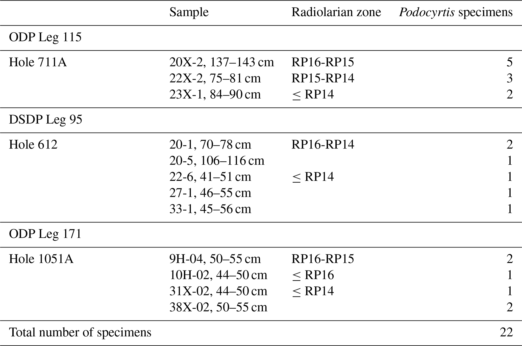
A total of 1085 radiolarian specimens were selected from the material available from the Demerara Rise. Their images were taken and prepared at the University of Lille and used for both training and validation of the CNN. The number of specimens used per species varies between 46 and 288 (Table 1). A second testing set of samples was prepared with 22 specimens that are stored at the Museum für Naturkunde in Berlin (see Table 2). Ten of them come from the Indian Ocean (Madingley Rise, ODP Leg 115, Hole 711A, Shipboard Scientific Party, 1988), six other specimens come from the western North Atlantic Ocean (New Jersey slope, Deep Sea Drilling Project (DSDP) Leg 95, Hole 612, Shipboard Scientific Party, 1987) and six others also from the western North Atlantic Ocean (Blake Nose, ODP Leg 171B, Hole 1051A, Shipboard Scientific Party, 1998).

3 Methods

We followed two different approaches for collecting photographs of specimens of Podocyrtis with the aim of constructing image datasets. A first approach involved the use of radiolarian slides from Leg 207, Hole 1260A, prepared initially for a biostratigraphic examination. The second involved the collection of Podocyrtis specimens, picked up directly and individually from dried residues of washed samples coming from both Holes 1260A and 1259A. The challenge faced while taking images of Podocyrtis from the old slides consists in specimens often touching themselves or overlapping with other objects. This led as a consequence to individual Podocyrtis specimens not being segmented properly by the methods described below and requiring manual (and time-consuming) segmentation.

3.1 Manual picking of individual Podocyrtis specimens

The residues used for sample preparation had already undergone acidic cleaning and removal of other non-siliceous particles by first dissolving the samples in hydrogen peroxide and afterwards in hydrochloric acid, followed by sieving at 50 µm. Some of the samples needed further sieving to remove particles smaller than 45 µm. They were then dried in a 50–60 ^∘C oven.

Specimens of the various species of Podocyrtis were manually picked one by one under a ZEISS SteREO Discovery V20 microscope. The radiolarians were then transferred to a 32×24 mm coverslip and placed in such a way so as to avoid them being in contact with each other. A few drops of distilled water were placed on the coverslip for radiolarians to attach to the coverslip. Thereafter, they were dried overnight in an approximately 50 ^∘C oven and thereafter attached on slides with Norland epoxy.

Table 2 Number of specimens per species for each sample coming from ODP Leg 115, DSDP Leg 95 and ODP Leg 171, which were used for the test.

3.2 Image acquisition and processing

Images of Podocyrtis were taken under a Zeiss Axio A2 transmitted light microscope using the Zen 3.2 software with ×100 magnification and a pixel size set to 0.35 µm per pixel. Images were taken in fields of view (FOV), enabling several radiolarians to be captured at once in the same FOV. Approximately 3–15 focal points were taken on each FOV, depending on the specimen size. The images were then stacked using Helicon Focus 7 (Fig. 3a–c). They were then segmented (i.e., isolated from the background) all at once (Fig. 3c–d) using the ImageJ BioVoxxel plugin (Brocher, 2022) and a modified version of the Autoradio_Segmenter plugin (Tetard et al., 2020).

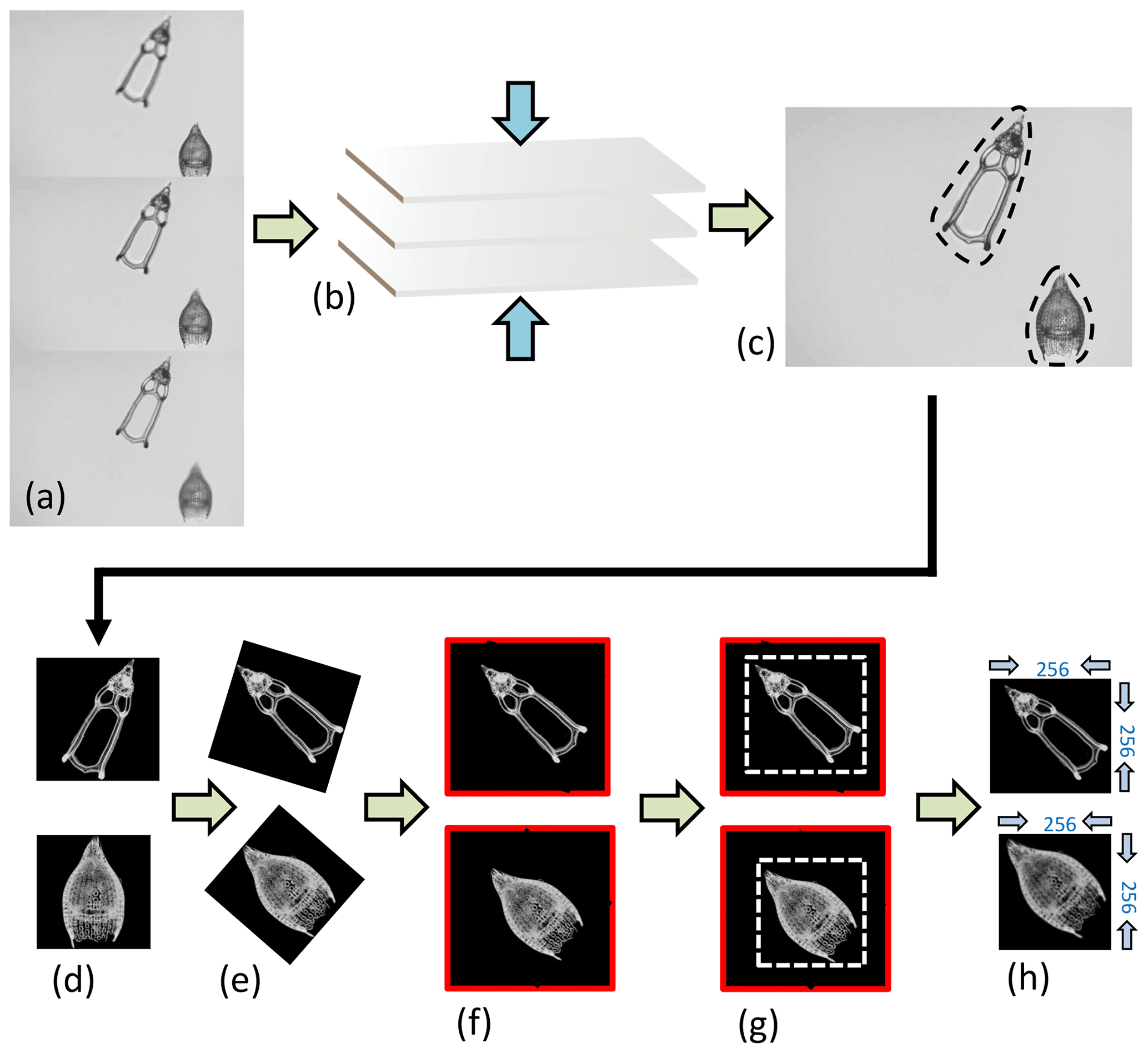
Figure 3 Image processing. (a) Three “raw” images taken from the microscope from the same FOV but from different focal points, which are (b) stacked together using the Helicon Focus 7 software (c) to produce one entire focused and crisp image in which each particle in one FOV is segmented into an individual image or so called vignette. (d) The segmented images are also transformed into a square 8-bit grayscale with a black background and white objects that are (e) further processed in Python by first rotating the radiolarian objects in the vignettes with a 45^∘ angle so that the longest axis goes from the upper left corner to the lower right corner. (f) The vignettes are then filled again into squares so that no parts of the specimens are removed. (g) Thereafter, they are cut again into squares just precisely so that the specimen fills the entire square and, lastly, the new images are resized to 256 pixels on each side image (h).

The images were then further processed with a script from Scikit Image version 0.18.1 (Van der Walt et al., 2014), using Python version 3.7.10 (Van Rossum and Drake, 2009), which rotated them in the same direction along a diagonal angle by finding the longest axis on the radiolarian specimen without cutting off objects within the picture (Fig. 3d–h). Thereafter, all images were resized to equal 256×256 pixels. Having all images in the same orientation decreases the variability and increases the accuracy of the neural network. By having the images rotated in a diagonal angle optimizes the pixel resolution.

The most time-consuming task is the collection of images, as numerous images are needed for each species to build up a consistent dataset. Automatization of this task may be facilitated by the use of an automatic microscope, as in Itaki et al. (2020), Tetard et al. (2020) and Marchant et al. (2020).

The time needed for picking, slide mounting, photographing and image processing of around 100–200 radiolarians was one day. Manual picking speeds up the process, although caution should be exercised to add glycerin or gelatin instead of water while mounting individually picked radiolarians on coverslips, in order to avoid formation of bubbles.

3.3 Datasets

The radiolarian specimens included in the training and validation datasets contain only individuals that display a variability that may be included in the morphological boundaries accepted in the concept of each one of the eight species. Specimens that could not be identified with certainty as one or the other morphospecies (i.e., intermediate forms) were removed. All images are in full focus or so called “stacked”. The images were divided into three different leveled datasets: the “normal” stacked dataset, called the “S” dataset (Fig. 4); the “SC” dataset, with only complete (unbroken) specimens, which obviously contains fewer radiolarian specimens but images of good quality; and the “SCUB” dataset, for which all blurry images were removed from the “SC” dataset (Fig. 4).

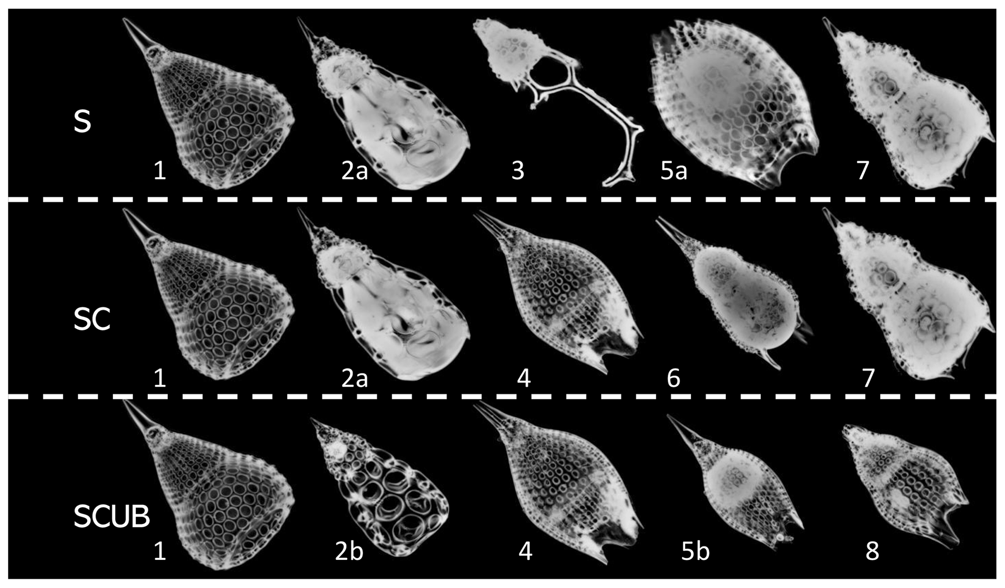
Figure 4 Images of fully processed specimens (vignettes) with stacking, segmentation, rotation and resizing. (1) P. ampla. (2) P. chalara. (3) P. goetheana. (4) P. papalis. (5) P. diamesa. (6) P. phyxis. (7) P. mitra (P. trachodes). (8) P. sinuosa. “a” and “b” stand for different individuals. S = stacked dataset. SC = stacked dataset with only complete specimens and SCUB = stacked dataset with only complete and unblurred specimens.

In all these datasets, 85 % of all specimens were used for training the model and 15 % of all specimens were only used to validate the trained neural network with the train and test split function from Scikit-learn (Pedregosa et al., 2011). This distribution aims to keep enough images to have quality learning, while having enough images for the network assessment to make sense of and to avoid miscalculations by running the model several times. Since the training and validation sets were randomized each time, it was important to perform several runs and thereafter take note of an average accuracy value. Neural network performance was compared between these different datasets.

3.4 MobileNet convolutional neural networks

The CNNs are constructed by node layers including input layers which transfer their information in the form of node connections with different weights and threshold values into hidden layers, the convolutional layers, which process and transform the information into the next layers. Each convolutional layer has a different size and number of filters. A filter can be seen as a small grid of pixels, with different pixel values in each grid corresponding to a specific color value. This grid will go through an entire image in a sliding (convolving) way and transform the new values to the next layer that will process the image in a different or similar way. Early layers could, for example, easily detect edges, circles or corners, and later layers can even recognize more specific objects (Krizhevsky et al., 2012).

The network used for training specimens in classification is the Keras implementation of MobileNet (Howard et al., 2017), which is a convolutional neural network architecture (Chollet, 2015). Since MobileNet is a relatively small model, less regularization and data augmentation procedures are needed because smaller models have fewer problems with overfitting (Howard et al., 2017).

The input size of the images in the network was set to $\mathrm{256}\times \mathrm{256}\times \mathrm{3}$ (number three stands for red, green and blue (RGB) colors or channels), dropout was set to 0.15 for layers trained by ImageNet inside the MobileNet architecture and an average pooling was used. An added dropout layer was set to 0.5 and added after the MobileNet convolutional layers to prevent overfitting by randomly switching off some percentages of neurons in the model. Finally, a dense layer was added, which is the most commonly used layer in neural network models. It performs a matrix-vector multiplication, for which values are parameters and which can be trained and updated with backpropagation, and the dense layer was set to eight outputs corresponding to the number of species. The SoftMax activation used here converts the values into probabilities. The optimizer used was “Adam”, a stochastic gradient descent, and the loss function used was “Categorical Crossentropy”. The batch size of 64 resulted in 100 steps per epoch and only three epochs were necessary for the training, for the simple reason of avoiding any overfitting models. After three and sometimes four epochs, the validation accuracy does not increase further, and the loss becomes bigger (see Tables S1–S3 in the Supplement 1 for an example of a MobileNet run on five epochs). For each dataset, since we used the train–test split function, the model was run 10 times to obtain good enough average accuracies.

4 Results

4.1 CNN accuracies

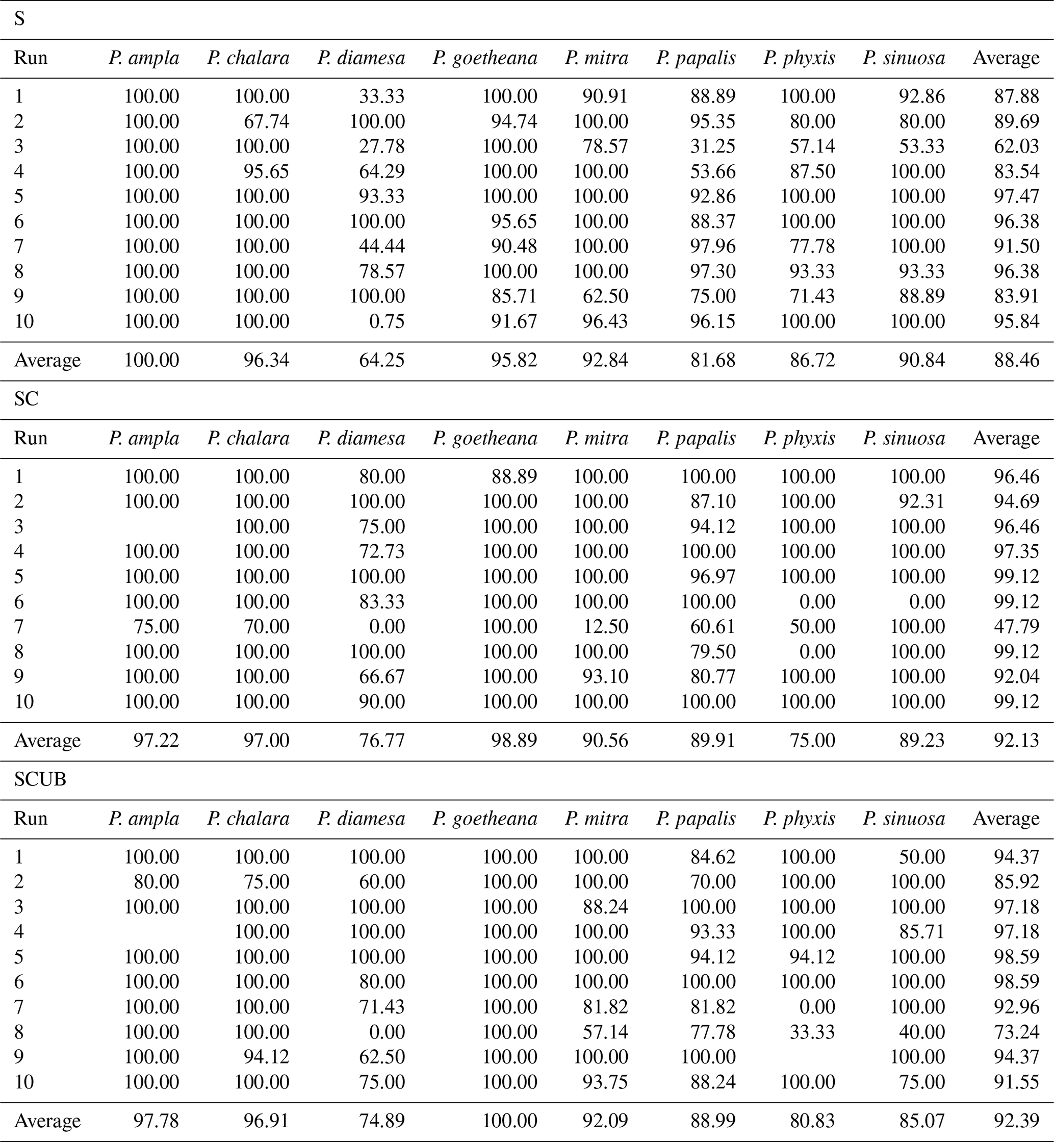
The MobileNet convolutional neural network model used here resulted in an average validation accuracy of 88.46 % for 10 runs of the “S” dataset, 92.13 % average accuracy for the “SC” and 92.39 % for the “SCUB” datasets for 10 runs on each dataset (Table 3). It is important to investigate how each run was performed, since it may vary a lot, especially by looking at each individual species' performance (Table 3). Although there are codes that can equally select 15 % from each species, we chose not to use that option here because we also wanted to see how the model performs without selecting all general forms for each species. The total time to run MobileNet on all datasets (total of 30 times) was around 8.5 h, 10–15 min for each run. In general, the “S” dataset with complete specimens had the smallest difference between the lowest and highest accuracies over its 10 runs. The dataset consisting of stacked, complete, clear and crisp specimens also had low variation between the highest and lowest accuracies.

Table 3 Validation accuracies for all the studied species over 10 runs for each one of the three datasets, and their average values based on the results of the species accuracies from Supplement 2.

4.2 Confusion matrices

The neural networks also produced confusion matrices for each run. Since the training and validation sets were randomized, we therefore created three average confusion matrices (Fig. 5), one for each type of dataset. Since the number of specimens used for validation varies, we calculated an average value for the validation size as well. In these confusion matrices the y-axis shows the actual species, while the x-axis shows predicted ones. Each box shows the average accuracy based on the validation set.

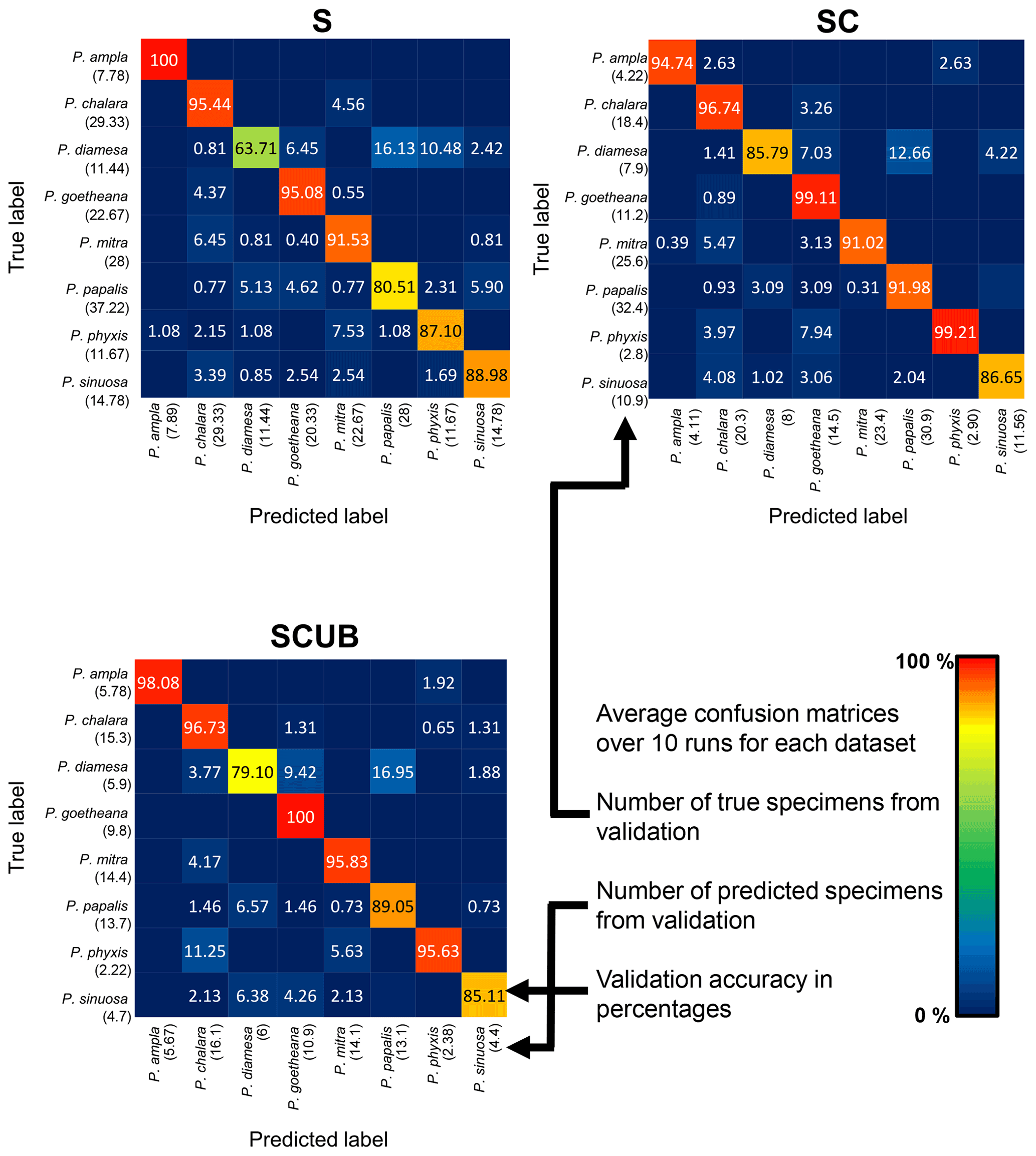
Figure 5 Average confusion matrices for the “S”, “SC” and “SCUB” datasets. The numbers inside the matrices show the average validation accuracy of specimens in each class that has been correctly or incorrectly classified. The numbers under each species name are the total number of true or predicted labels.

What is further observed is the fact that closely related species (i.e., morphospecies situated along an evolutionary lineage) are often mistaken for each other. This is true especially for those species with more than one neighboring species along a lineage, which is the case for all species studied here with the exception of the lineage end members, e.g., P. ampla and P. goetheana. A very remarkable point is that P. diamesa appears to often be misidentified as P. papalis, more frequently than P. papalis is misinterpreted as P. diamesa, which results in the average precision value being lower in P. diamesa compared to the rest of the species, while P. papalis has a lower recall than precision value.

Figure 6 displays the calculated average precision, recall and F1 score for all species based on the confusion matrices. The precision value also means the correct prediction value, and can be simplified by the following Eq. (1):

$$\begin{array}{}\text{(1)}& \text{Precision}={\displaystyle \frac{\begin{array}{c}\mathrm{\text{Number of specimens classified as a class}}\\ \mathrm{\text{and also belonging to that class}}\end{array}}{\begin{array}{c}\mathrm{\text{All specimens classified}}\\ \mathrm{\text{as that particular class}}\end{array}}}.\end{array}$$

The recall values show that not all specimens belonging to a class have been classified to the correct class, similar to the accuracy, which is the number of specimens correctly classified divided by the total number of specimens, as in the Eq. (2):

$$\begin{array}{}\text{(2)}& \text{Recall}={\displaystyle \frac{\begin{array}{c}\mathrm{\text{Number of specimens in a class that}}\\ \mathrm{\text{were correctly classified}}\end{array}}{\text{Total number of specimens in that class}}}.\end{array}$$

The F1 score is an average value of this and shows the average between precision and recall written like Eq. (3):

$$\begin{array}{}\text{(3)}& \text{F1}={\displaystyle \frac{\mathrm{2}\cdot (\mathrm{precision}\cdot \mathrm{recall})}{\mathrm{precision}+\mathrm{recall}}}.\end{array}$$

The average F1 scores based on the confusion matrices are 89.05 %, 93.26 % and 91.72 % for the “S”, “SC” and “SCUB” datasets, respectively. This implies that the best result for the F1 score is obtained when the CNN was trained on the “SC” dataset.

Figure 6 Average precision, recall and F1 score calculated from the average confusion matrices based on the S, SC and SCUB datasets.

4.3 Testing the predictive models

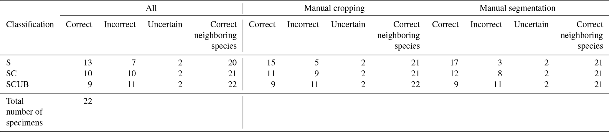
Once a high validation accuracy (i.e., over 90 %) had been obtained for each dataset following the training process, parameters were saved and predictive models were formed. The idea is to explore how the classification tool classifies Podocyrtis species and with what level of confidence. Therefore, a total of 22 specimens of Podocyrtis obtained from ODP Leg 171B, Hole 1051A (Blake Nose, western North Atlantic Ocean), DSDP Leg 95, Hole 612 (New Jersey slope, North Atlantic Ocean) and ODP Leg 115, Hole 711A (Madingley Rise, Indian Ocean) were used as a test dataset. Slides were prepared with Canada balsam and photographs were taken with a Leica transmitted light microscope to which an AmScope MU1003 digital camera was attached. Images were then segmented with ImageJ, and rotated and resized with a Python script as described above. Some images were further cropped, but no background particles were removed. Tables S4–S6 in Supplement 1 display how each specimen from the different locations was classified using different predictive values, a comparison with classification by cropping images that appeared very tiny in relation to the entire image and a comparison of removing background particles of those specimens which displayed them. The main result shows that P. sinuosa is often misinterpreted as P. papalis even though P. papalis is almost always classified correctly. There are significant morphological differences between the species trained in the neural network and the test set. Here, the best predictive model to use is the “S” dataset and the worst one is “SCUB” (Table 4), which is quite the reverse from the validation set based on the tropical Atlantic specimens from the Demerara Rise trained in this network.

Results obtained after the model “S” was applied on material from the North Atlantic and Indian Oceans were 13 out of 22 specimens classified correctly without any manual fixation, which corresponds to 59 % accuracy. The accuracy of model “SC” was raised to 68 % after manually cropping images for specimens that appeared smaller, while it was increased up to 77 % by removing background particles appearing in the images. The “SC” model produced worse results. For all images without any manual fixation, the accuracy obtained was 45 %, but increased up to 50 % after adding manual cropping and to 54.5 % after adding the segmentation. The “SCUB” model had an accuracy of 41 % for all three of the different image fixations. However, in all cases, in terms of neighboring species, at least 20 specimens were correctly classified as a neighboring species which translated into an accuracy of at least 90.9 %.

Table 4 Results of all the 22 specimens including necessary manual cropping and segmentation from ODP Leg 115, Hole 711A from the Indian Ocean; DSDP Leg 95, Hole 612; and ODP Leg 171, Hole 1051A from the western North Atlantic Ocean which were classified using different parameters trained on the three different datasets “S”, “SC” and “SCUB”.

5 Discussion

5.1 MobileNet performance and accuracy

Dedicated to embedded systems and smartphones for which low latency and real-time execution are key demands, the advantage of using the MobileNet architecture is that it is extremely light and small (in terms of coding and weight of models). It is fast, with an only slight degradation in inference accuracy according to the gain of the consumed resources, and easily configurable to improve detection accuracy (Howard et al., 2017). When tested on Im2GPS, a dataset which gives geolocation from images taken from different spots around the world, the accuracy of MobileNet was about 1 % higher compared to GoogleNet, whereas it used 2.5 times less computation and, as cited in Howard et al. (2017), “MobileNet is nearly as accurate as VGG16 while being 32 times smaller and 27 times less compute intensive”. The study by Howard et al. (2017) presents extensive experiments on resource and accuracy trade-offs and shows strong performance of MobileNet compared to other popular models on ImageNet classification. This is the reason why some works (Rueckauer et al., 2021) start to deploy MobileNet also on neuromorphic hardware such as Loihi (Davies et al., 2021). Although the development of AI has been based until now on software bricks installed on big data centers, the current multiplication of connected objects requires decentralization. The new AI revolution now involves development of specific electronic components with very promising results.

The images that we have used were transformed to RGB-colored because the pretrained weights of ImageNet are only compatible for RGB-colored images, as this is also the case of the whole architecture of MobilNet; the idea here is to apply a depthwise convolution for a single filter for each unique input channel. The use of neural network models, equally adapted for grayscale images, could also decrease the energy consumption greatly. In terms of resolution, MobileNet resizes images into a lower resolution. In most cases this did not affect the result, but it is plausible that in a few cases the neural network was not able to see the position of the lumbar stricture, which is an important distinguishing character. In any case, Renaudie et al. (2018) also commented on the resolution loss due to resizing, as the inner spicules in Antarctissa species disappeared, which are crucial for species identification.

The species with the highest F1 score (Fig. 5) were P. goetheana (94 %–97 %) and P. ampla (90 %–99 %). A reason for this might be that both species are at the end of the Lampterium and Podocyrtoges lineages and have only one closely related species, while the others have two. For P. chalara, P. sinuosa and P. mitra, a reduction in the number of analyzed specimens increased the precision and increased the recall value for P. mitra, giving P. mitra an overall better F1 score with reduction of specimens. This is expected, since the variability decreases when removing more imperfect specimens but performs better for determining unbroken and clear specimens. A reduction of specimens for P. goetheana did not make a big difference to precision but it did increase the recall. In general, P. diamesa has both the lowest recall (69 %–85%) and precision (80 %–84%) values. Although P. diamesa and P. papalis are often mistaken for one another, it is mostly P. diamesa that is misidentified as P. papalis, which may be due to the fact that late morphotypes of P. papalis resemble P. diamesa to some extent. The distinguishing character of this species is that the overall shape of P. papalis is in most cases rather fusiform with a larger thorax than abdomen, which is only partially developed. Podocyrtis diamesa is much larger (even though this does not seem to matter since all images are resized to equal sizes), the size of the thorax and abdomen is often more similar, and the lumbar stricture is more prominent. Although late forms of P. papalis do resemble P. diamesa, they do not co-exist at the same time interval (the true P. diamesa morphospecies disappeared well before the appearance of the late P. papalis forms) and they are smaller.

The highest F1 score for all species except P. diamesa comes from using a model trained on complete specimens (“SC”), regardless of quality. Podocyrtis phyxis is one example of a species that has the best performance in the “SC” dataset. The overall dataset of P. phyxis consists of many specimens that are broken and missing the apical horn; therefore, there is a significant reduction of specimens when using the datasets with only complete specimens. The number of specimens present for P. phyxis in the “S” dataset was 64. This number dropped down to 22 specimens in the “SC” dataset and then further to 16 specimens in the “SCUB” dataset. When it comes to P. sinuosa, there is a substantial reduction due to many blurry specimens, which is likely the result of the mounting media. A total of 49 blurry specimens were removed from the “SC” dataset (78) compared to the “SCUB” dataset (29), and the overall result seems to have been improved somewhat by removing specimens.

To summarize, our work has about 91 % accuracy if we exclude the tests run with the unstacked (U) dataset (Supplement 1, Table S7), which not only consisted of blurry unfocused images but also kept some touching particles. Nevertheless, it has an overall similar accuracy of about 72 % to the work produced by Renaudie et al. (2018) with the same neural network. These authors used images as they appear under the microscope, without stacking or image processing. To produce more datasets with these types of images, one can expect a slightly lower accuracy than when images are processed. Renaudie et al. (2018) also included a substantial number of unidentifiable specimens. If these unidentifiable images were ignored, results would probably come close to 90 % accuracy. In our case, all specimens are identifiable by our CNN as any of the eight possible Podocyrtis species, even if the specimen in question is not a Podocyrtis. A solution for this issue is to perhaps apply parallel neural networks with a hierarchical architecture, similar to the one that Beaufort and Dollfus (2004) applied for SYRACO. One suggestion could be first to classify radiolarians and non-radiolarian particles, with a second step classifying radiolarians into higher taxonomic orders (Spumelleria, Nassellaria and unidentified broken radiolarians) and finally, a last step leveling down to species, genus and/or family levels. Itaki et al. (2020) went with another approach. These authors focused on the identification of one single species, Cycladophora davisiana, but they also used the morphologically similar species, Cycladophora bicornis, as another class, to avoid this species being wrongly interpreted as C. davisiana. Thereafter, they used the classes “centric diatoms”, “all other radiolarians” and “all other objects”.

It is worth noting that validation accuracies and F1 score values may appear high since we do not have a large dataset and the images in the datasets are in the same orientation and rotational angle, centralized in the middle. As mentioned earlier, species are carefully selected to avoid including any intermediate forms in the dataset.

5.2 Predictive models

Given that our initial analysis was performed with material coming from the equatorial Atlantic (ODP Leg 207), we wished to consider a different dataset to test the predictive models, which consisted of images of specimens coming from the North Atlantic (DSDP Leg 95, ODP Leg 171) and the Indian Ocean (ODP Leg 115). In addition, radiolarians were mounted in a different mounting media (Canada balsam) and we used a different microscope. In most cases, particles were segmented properly in the segmentation process. However, some specimens were still attached to other particles, which could also result in that the specimens did not fill out the entire images. To save time and effort, we did not crop or remove background particles at first. These specimens could still be classified correctly. The results improved after the specimens were cropped or had their background particles removed, at least by using the predictive model trained by the “S” dataset. Podocyrtis papalis is almost always correctly interpreted. The reason might be the large number of specimens used in our dataset and the large number of morphological differences within the species. As mentioned earlier P. sinuosa is often misinterpreted as P. papalis. This is almost always the case for all P. sinuosa, whether we use the “SC” or “SCUB” datasets. The main reason for this probably lies in the fact that the morphotypes of P. sinuosa coming from the North Atlantic and the Indian oceans differ significantly (Fig. 2) from the ones trained in the initial neural network. Two other factors may contribute to this: first the decrease in P. sinuosa specimens when passing from the “S” dataset to the “SC” and “SCUB” datasets, as explained above; and secondly, the image quality, since P. sinuosa appear very whitish in the trained neural network. One P. chalara was first classified as P. mitra before it was cropped. One possible reason may have been that the pores of the uncropped version appeared smaller, as in P. mitra. After cropping out unnecessary space, P. chalara appeared larger and could be correctly classified. In one case, one specimen, which was clearly a late P. mitra (according to preference of the author and not P. trachodes), was completely wrongly identified as either P. phyxis by using the “S” predictive model, P. ampla by using the “SC” predictive model or P. goetheana by using the “SCUB” predictive model. The reason for this may be due to the mounting media or preservation, because the pore space appears blacker or cleaner, similar to P. phyxis or P. ampla, which are generally larger from the tropical Atlantic assemblages trained in this network, and resizing the images may make them appear to be in a better resolution, with no white “dirt” between the pores and within the pore space. Podocyrtis goetheana also have gigantic pores and a lot of black space.

Most often it is closely related species that are mistaken for each other, as observed in the training and validation. It can be observed in Table 4 that even if specimens were not always interpreted as the right species, they were almost always interpreted as a neighboring species along a lineage. It was also discussed by Renaudie et al. (2018) that closely related species tend to be misinterpreted as each other due to morphological similarities, which is also confirmed in this work.

5.3 Species choice and their image properties

Akin to the study of Renaudie et al. (2018) conducted on Neogene radiolarians, we used the MobileNet neural network to classify closely related species of the Eocene genus Podocyrtis. We did not, however, use images as they appeared under the microscope, since we used software and codes for image processing which can easily process several images into equal settings at once and do not only increase the image quality but also save a lot of time and effort.

Renaudie et al. (2018) chose to select all specimens present in a slide that could somehow be classified with reliable confidence. The same approach was followed here, but most of the samples were pre-selected knowing that some typical morphotypes existed in them. We used specimens for which species identification and classification was certain in most cases, meaning specimens which could be instantly recognized to one species, and left out uncertain intermediate forms. We also used specimens which were preserved nearly completely, even though many experts are often able to identify specimens based on even small fragments to at least a genus level. Smaller identifiable fragments would probably require a huge amount of data to train. The samples obtained here have excellent preservation and finding broken fragments in, for example, dinoflagellate cysts seem more likely than finding broken pieces of radiolarians, provided they have not been crushed by mounting.

6 Conclusions

The goal of this study was to create an automatic classification tool to allow AI-based identification of middle Eocene Podocyrtis species which would achieve the highest possible accuracy after training the MobileNet CNN based on a dataset of 1085 images of Podocyrtis morphotypes classified as eight different species.

Regarding our first question stated in the introduction, “How well can the MobileNet convolutional neural network classify closely related species of the genus Podocyrtis?”, we showed that specimens which belong to Podocyrtis species can be classified automatically with a high accuracy (91 % confidence). Best results were obtained by using datasets with improved quality (but a smaller number of images), both according to overall accuracy and the F1 score values. However, tests on Podocyrtis species from the North Atlantic and Indian Ocean work best by using the predictive model trained by the normal stacked dataset, consisting of more specimens but with a mix of broken, complete, blurry and clear images. This suggests that a higher variance of morphotypes could be applied to the datasets. In conclusion, this identification tool works well for classification of Podocyrtis species, although it could still be further improved by adding additional closely resembling species of Podocyrtis that were not present or very rare in our material.

Regarding our second scientific question, “How well can the predictive model classify Podocyrtis species under different processing settings and using material coming from different parts of the world's oceans?”, we establish that the predictive models also work well for classifying images taken by different microscopes, but might in some cases require adjustment of the clarity settings and images taken by different mounting medias.

This study could be further improved by including additional morphospecies of Podocyrtis in the datasets and more specimens and morphotypes, especially from many other different oceanic realms. Another improvement to the neural network would be to detect Podocyrtis species or other taxa of interest among hundreds to thousands of other objects. This could perhaps be solved by classifying every object, as, for example, done in Tetard et al. (2020) and Itaki et al. (2020), or by applying a parallel network approach (Beaufort and Dollfus, 2004) first that filters away objects of no interest in different steps. For example, as a first step, this would involve the classification of radiolarians and non-radiolarians, and as a second step, the exclusion of all non-radiolarians. It could also be beneficial to create a network inspired by MobileNet but adapted to grayscale images, in order to become more energy efficient and have a more appropriate resolution that detects small crucial details in radiolaria classification.