the Creative Commons Attribution 4.0 License.
the Creative Commons Attribution 4.0 License.
 | 02 Jun 2023
An expanded database of Southern Hemisphere surface sediment dinoflagellate cyst assemblages and their oceanographic affinities
Lena Mareike Thöle
Peter Dirk Nooteboom
Suning Hou
Rujian Wang
Senyan Nie
Elisabeth Michel
Isabel Sauermilch
Fabienne Marret
Francesca Sangiorgi
Dinoflagellate cyst assemblages present a valuable proxy to infer paleoceanographic conditions, yet factors influencing geographic distributions of species remain largely unknown, especially in the Southern Ocean. Strong lateral transport, sea-ice dynamics, and a sparse and uneven geographic distribution of surface sediment samples have limited the use of dinocyst assemblages as a quantitative proxy for paleo-environmental conditions such as sea surface temperature (SST), nutrient concentrations, salinity, and sea ice (presence). In this study we present a new set of surface sediment samples (n=66) from around Antarctica, doubling the number of Antarctic-proximal samples to 100 (dataset wsi_100) and increasing the total number of Southern Hemisphere samples to 655 (dataset sh_655). Additionally, we use modelled ocean conditions and apply Lagrangian techniques to all Southern Hemisphere sample stations to quantify and evaluate the influence of lateral transport on the sinking trajectory of microplankton and, with that, to the inferred ocean conditions. k-means cluster analysis on the wsi_100 dataset demonstrates the strong affinity of Selenopemphix antarctica with sea-ice presence and of Islandinium spp. with low-salinity conditions. For the entire Southern Hemisphere, the k-means cluster analysis identifies nine clusters with a characteristic assemblage. In most clusters a single dinocyst species dominates the assemblage. These clusters correspond to well-defined oceanic conditions in specific Southern Ocean zones or along the ocean fronts. We find that, when lateral transport is predominantly zonal, the environmental parameters inferred from the sea floor assemblages mostly correspond to those of the overlying ocean surface. In this case, the transport factor can thus be neglected and will not represent a bias in the reconstructions. Yet, for some individual sites, e.g. deep-water sites or sites under strong-current regimes, lateral transport can play a large role. The results of our study further constrain environmental conditions represented by dinocyst assemblages and the location of Southern Ocean frontal systems.
- Article
(9521 KB) - Full-text XML
-
Supplement
(457 KB) - BibTeX
- EndNote


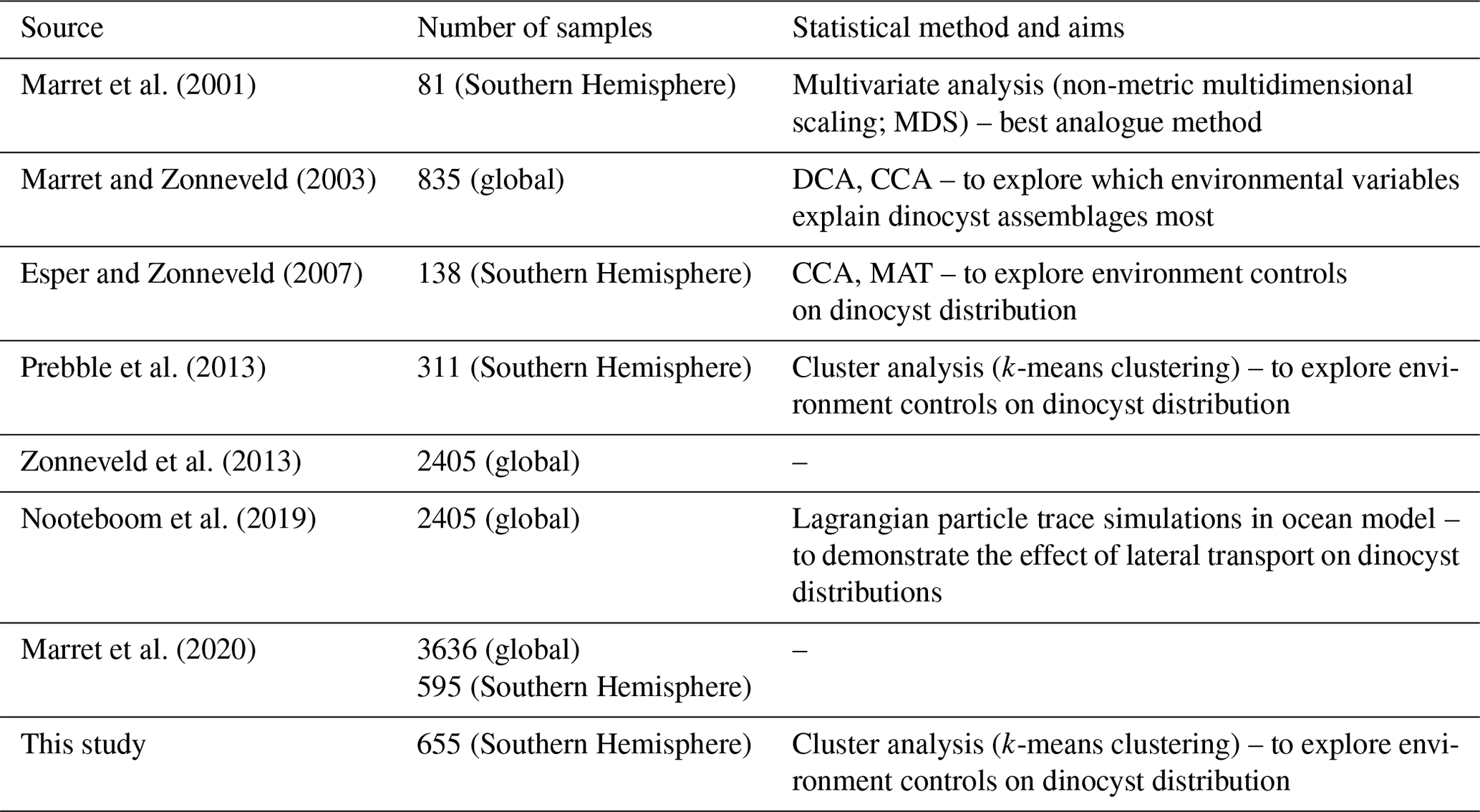
Dinoflagellate cyst assemblages have been increasingly used as a proxy to reconstruct southern high-latitude oceanographic conditions for the late Paleogene to recent (34–0 million years ago; Esper and Zonneveld, 2007; Prebble et al., 2016; Sangiorgi et al., 2018; Bijl et al., 2018a; Hoem et al., 2021a, b; Marschalek et al., 2021). Such reconstructions rely on an accurate understanding of the modern ecological affinities of taxa. For extant species, modern biogeography is statistically linked to surface oceanographic conditions (sea surface temperature, nutrients, salinity, sea ice; de Vernal et al., 2005; Zonneveld et al., 2013; Prebble et al., 2013; Mudie et al., 2017; Marret et al., 2020; see Table 1 for an overview). They all assume that the assemblages in a surface sediment sample at a certain location represent the parameters of (and are derived from) the sea water directly above the sediment. Transfer function techniques then offer a quantitative approach to directly translate (down-core) assemblages into values of past environmental parameters (e.g. Marret et al., 2001; de Vernal et al., 2005; Esper and Zonneveld, 2007). This requires a sufficiently large training set, with a large number of geographically widespread surface sediment samples, so that the full variety of surface oceanographic conditions is represented.
Constraining oceanographic affinities of dinocyst species has been hindered by the low number and uneven geographic distribution of surface sediment samples from the Southern Ocean, particularly when compared to that in the Northern Hemisphere high latitudes (de Vernal et al., 2001, 2020). Notably scarce are samples from the Antarctic margin, i.e. the region south of the Polar Front (PF) (Marret et al., 2020). Among the most dominant species found close to the Antarctic margin, Selenopemphix antarctica is generally an environmentally significant taxon that is commonly associated with (past) Southern Ocean sea-ice presence (Harland and Pudsey, 1999; Marret et al., 2001; Houben et al., 2013). Sporadic occurrences of S. antarctica north of the winter sea-ice edge (Esper and Zonneveld, 2007) may be linked to northward transport by surface and deep currents from the sea-ice zone (Nooteboom et al., 2019). However, the low number of samples analysed from close to the Antarctic margin makes the sea-ice affinity of S. antarctica poorly constrained. Specifically, it is unknown what the regional applicability of S. antarctica as a sea-ice indicator may be and whether whole dinocyst assemblages from sea-ice regions may be more suitable than a single species to constrain past sea-ice conditions.
Previous attempts to apply transfer functions with surface sediment samples from the Southern Ocean focused on sea surface temperature (SST) reconstructions (Marret et al., 2001; Esper and Zonneveld, 2007). Pleistocene dinocyst assemblages from the Subtropical Front in the Pacific Ocean yield realistic SST reconstructions for interglacial time intervals that are in agreement with other proxies but that are also colder than those obtained with other proxies for glacial intervals (Marret et al., 2001). This is largely due to the occurrence of S. antarctica in glacial phases, which results in a cold bias in the transfer function output (Prebble et al., 2016). The extensive surface sediment sample set from around New Zealand (Prebble et al., 2013) demonstrated that S. antarctica is a rare member of dinocyst assemblages in the subantarctic Pacific, and in that region, its presence cannot be easily explained by lateral transport (Nooteboom et al., 2019). This raises questions about whether this species lives exclusively in regions covered with sea ice. Esper and Zonneveld (2007) showed an overall good consistency in terms of dinocyst-based SST reconstructions compared to those from other proxies for Southern Ocean sediment cores spanning the past 140 kyr, with some potential bias due to selective degradation of dinocysts (Esper and Zonneveld, 2007).
Table 1Dinocyst compilation efforts. DCA – detrended correspondence analysis; CCA – canonical correspondence analysis; MAT – modern analogue technique.
Lateral transport of sinking particles creates a deviation from the first-order approximation that plankton (or other particles) found in the sediments relate to oceanographic conditions in the surface waters directly overlying the site (e.g. Zonneveld et al., 2013). For instance, Nooteboom et al. (2019) showed that lateral transport can affect the location of deposition under realistic assumptions regarding the sinking speed of pelagic particles in their descent towards the ocean floor. The effect of lateral transport on sinking particles is large in places with deep (>1 km) waters and strong currents, where currents flow meridionally (because that is the main direction of environmental gradients) and also where turbulence occurs during sinking (Nooteboom et al., 2019). Thus, the potential for lateral transport of pelagic particles should be considered when using sediment to assess surface water conditions at the site.
In this study, we present dinocyst assemblage data from a new surface sediment sample set predominantly from the Antarctic margin. This sample set fills a clear gap in previously underrepresented ice-proximal Southern Hemisphere surface sediment samples. Moreover, the wide geographic spread of these new samples allows for an investigation of longitudinal differences in ice-proximal dinocyst assemblages. Adding these to existing surface sediment samples of the Southern Hemisphere allows for an improved assessment of biogeographic and oceanographic affinities of Southern Hemisphere dinocyst assemblages. We compare dinocyst assemblages to the following oceanographic parameters: SST, salinity, nutrients (nitrate and silicate concentrations), and sea-ice cover. We assess these by analysing model output data, specifically for the surface water directly overlying the sites and for the surface water in the location of origin of the simulated particles that descended to those sites. This allows for an evaluation of the extent to which lateral transport affected the paleoceanographic affinities of sedimentary dinocyst assemblages.
2.1 The Southern Ocean
The dominant oceanographic feature in the Southern Ocean is the Antarctic Circumpolar Current (ACC; Marshall and Speer, 2012). Without land barriers and (partly) driven by strong Southern Hemisphere westerly winds, the ACC flows clockwise around Antarctica and is the world's strongest ocean current (>140 Sv; Orsi et al., 1995; Park et al., 2019, and references therein). The flow speed is the highest at the ocean fronts associated with the ACC, which introduces strong environmental gradients and creates quasi-latitudinal zones with characteristic environmental conditions (Fig. 1; Orsi et al., 1995). From north to south, the main fronts are the Subtropical Front (STF), the Subantarctic Front (SAF), and the Polar Front (PF; Fig. 1).
In general, the STF is considered to be the northern boundary of the ACC (Orsi et al., 1995). Surface water temperature changes by ∼ 4–5 ∘C and salinity changes by ∼ 0.5 across the 0.5∘ latitudinal band that represents the STF, which separates the warm, nutrient-poor subtropical surface waters of the subtropical gyres to the north from the colder and nutrient-rich subantarctic surface waters of the Subantarctic Zone to the south (SAZ; see Fig. 1).The SAF separates the SAZ from the Polar Frontal Zone (PFZ), where subantarctic surface waters are subducted to form Antarctic Intermediate Waters (Orsi et al., 1995). The PF separates these waters from the colder (<2 ∘C) Antarctic Surface Waters that form the Antarctic Zone (AZ). The typical high-nutrient, low-chlorophyll signature of the AZ is caused by a scarcity of light and by micro-nutrients which limit the utilization of available macro-nutrients. Overall, this leads to a dominance of silicate-based phytoplankton (e.g. diatoms) over calcareous species (e.g. coccolithophores). In the AZ, (seasonal) sea ice plays a major role, as it can strongly modulate light and nutrient availability (Mitchell et al., 1991). Sea ice is mostly found in areas close to the Antarctic continent, the Ross and Weddell seas, and Prydz Bay, where brine rejection promotes the formation of Antarctic Bottom Water, which then sinks to the deep ocean (Adkins, 2013; Talley, 2013; Solodoch et al., 2022).
Sea-ice dynamics differ between the Ross and Weddell seas. The Weddell Sea has a strong, dynamic gyre that transports sea ice and icebergs out of the Weddell Sea into the South Atlantic, an area known as Iceberg Alley (Orsi et al., 1995). The most prominent feature in the Ross Sea is the Ross Sea polynya, open patches in the sea ice, maintained by katabatic winds (Rhodes et al., 2009; Bromwich et al., 1992).
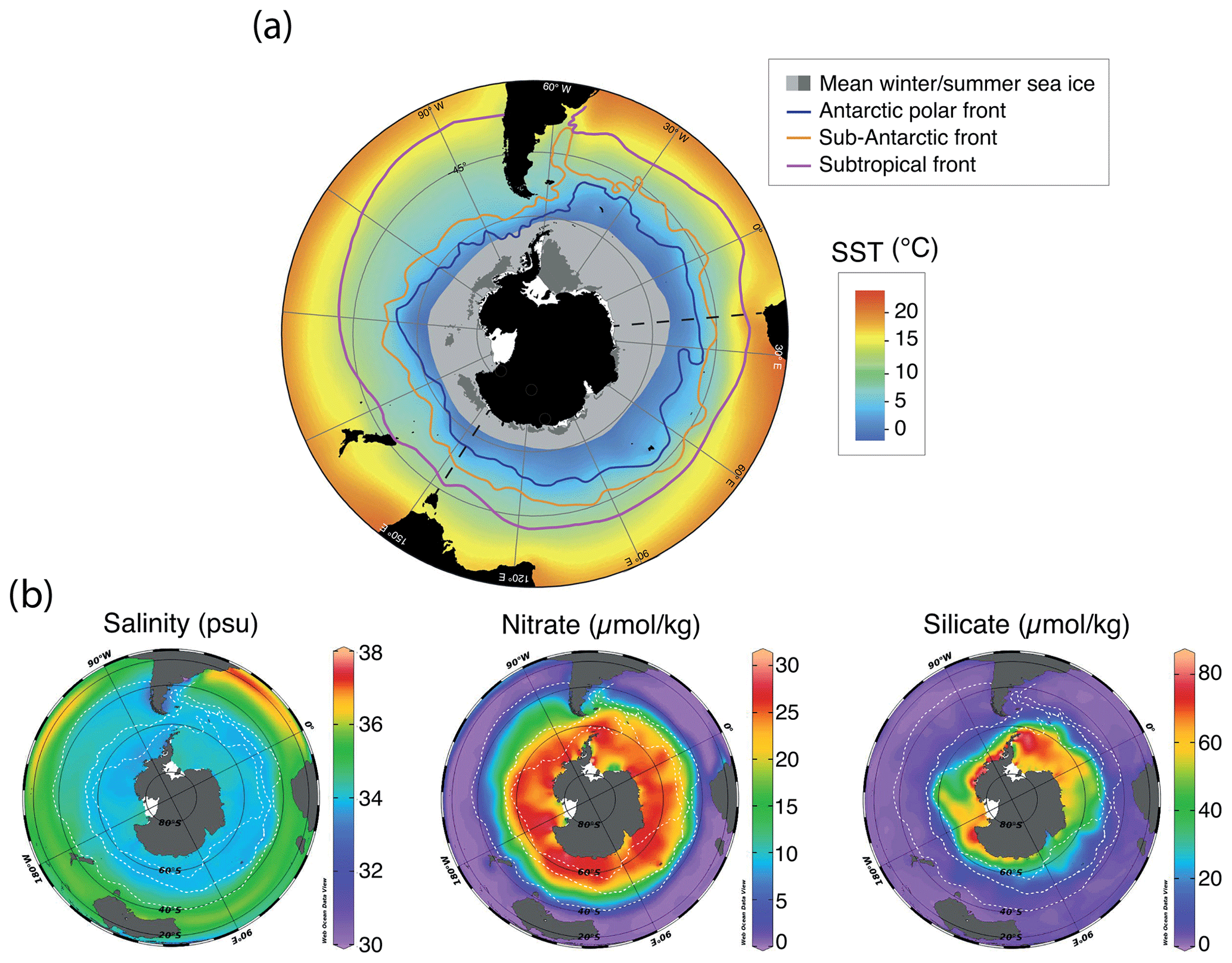
Figure 1Compilation of maps of modern annual average environmental parameters in the Southern Ocean. (a) Southern Ocean SST and approximate winter and summer sea-ice extent (modified from Crosta et al., 2021, and Spreen et al., 2015–2021). (b) Surface (1 m) salinity (psu) and nitrate and silicate concentrations (µmol kg−1). Data from the World Ocean Atlas (Locarnini et al., 2018). Maps were produced using ggplot2 in R (Wickham, 2016).
2.2 Lateral transport
Taking (past) lateral transport into account in the interpretation of sediment proxies remains difficult, as the quantification of transport comes with large uncertainties and assumptions regarding (past) ocean current strengths and directions, particle aggregation and size, and – connected to this – particle sinking speed (Nooteboom et al., 2019). Recent efforts have attempted to better constrain the influence of lateral transport on sedimentary microplankton assemblages by applying Lagrangian particle trace experiments in ocean model simulations with a spatial resolution high enough to represent an eddying flow (0.25∘ and finer; Nooteboom et al., 2019). In the Southern Ocean especially, it is thought that the ACC strength and sea-ice dynamics can assert a large influence on particle transport. Here, recent modelling efforts could explain unexpected, rare occurrences of species (Nooteboom et al., 2019) outside their common habitat. More specifically, findings of Selenopemphix antarctica north of the SAF could be attributed to latitudinal transport from the AZ, thus helping to better constrain and interpret the (past) ecological affinities of single species and to explain their rare presence in unexpected locations. This demonstrated the potential influence lateral transport may have in shaping microplankton assemblages and, through that, the inferred surface oceanographic affinities of microplankton species.
3.1 New surface sediment samples from around Antarctica
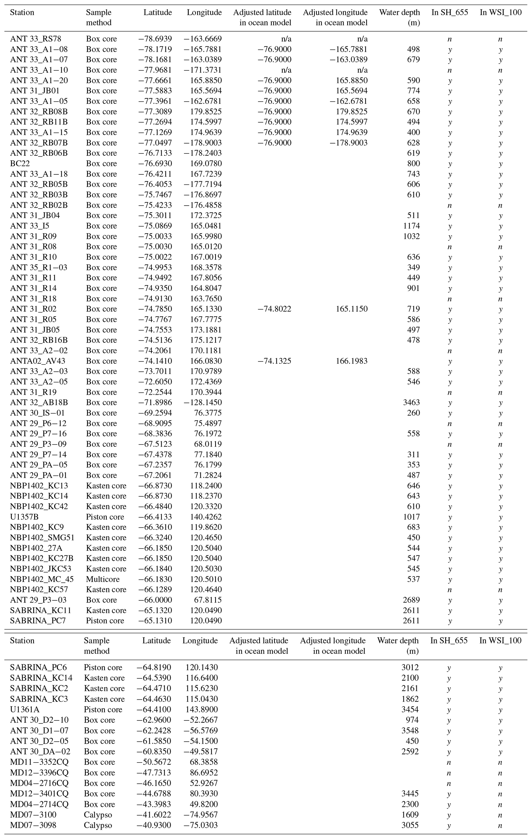
In total, we examined 66 new surface sediment samples located close to the Antarctic continent and 7 samples located north of the modern PF (Fig. 2; Table 2). For some new samples, existing age models confirm a modern or (Late?) Holocene age (e.g. Hartman et al., 2018; Wilson et al., 2018; Armand et al., 2018; Behrens et al., 2019). However, for many samples, no absolute age determination was available, but the use of the box-coring technique (Table 2) to retrieve the sediment–water interface together with the dinocyst assemblages and palynofacies found (e.g. the presence of more labile organic matter, such as amorphous organic matter and chitin remains) suggests a tentative modern-to-Late-Holocene age. Previous studies of modern surface sediments used an age cut-off of 7 ka (Prebble et al., 2013). We are confident that the data added here have a modern age similar to those of the data we compare ours to. We do note that this surface sediment sample set averages out potential environmental changes that occurred in the Holocene.
All samples, but particularly those from the Antarctic continental margin, may have been contributed to by reworked palynomorphs from older sediments (Bijl et al., 2018b). Most reworking is easily recognized (and excluded from further analysis) because these species are extinct. For extant taxa, such as Spiniferites ramosus, Operculodinium centrocarpum, and Nematosphaeropsis labyrinthus, it is impossible to assess from their appearance whether they are reworked or in situ. This means that caution should be taken when interpreting rare occurrences of these taxa.
A total of 46 productive samples are from south of 60∘ S and are located in the Ross Sea (28 samples), the Sabrina Coast (17 samples), Prydz Bay (6 samples), and the Weddell Sea (4 samples), almost doubling the number of existing samples from Antarctic ice-proximal sites to 100. We also add the first dinocyst assemblages from south of 70∘ S (Ross Sea, Fig. 2), yet some ice-proximal areas remain uncovered, such as the Weddell Sea and the offshore Dronning Maud Land, as well as most of the West Antarctic continental margin. The seven additional samples are from north of the PF, located close to Crozet Island, on the Kerguelen Plateau and along the west coast of South America (Fig. 2).
Most samples are in (relatively) close proximity to land, including the coast of New Zealand, the western coasts of southern Africa and Australia, and both sides of South America. The Atlantic has the highest spatial coverage, whereas the Pacific and Indian oceans appear to be underrepresented.
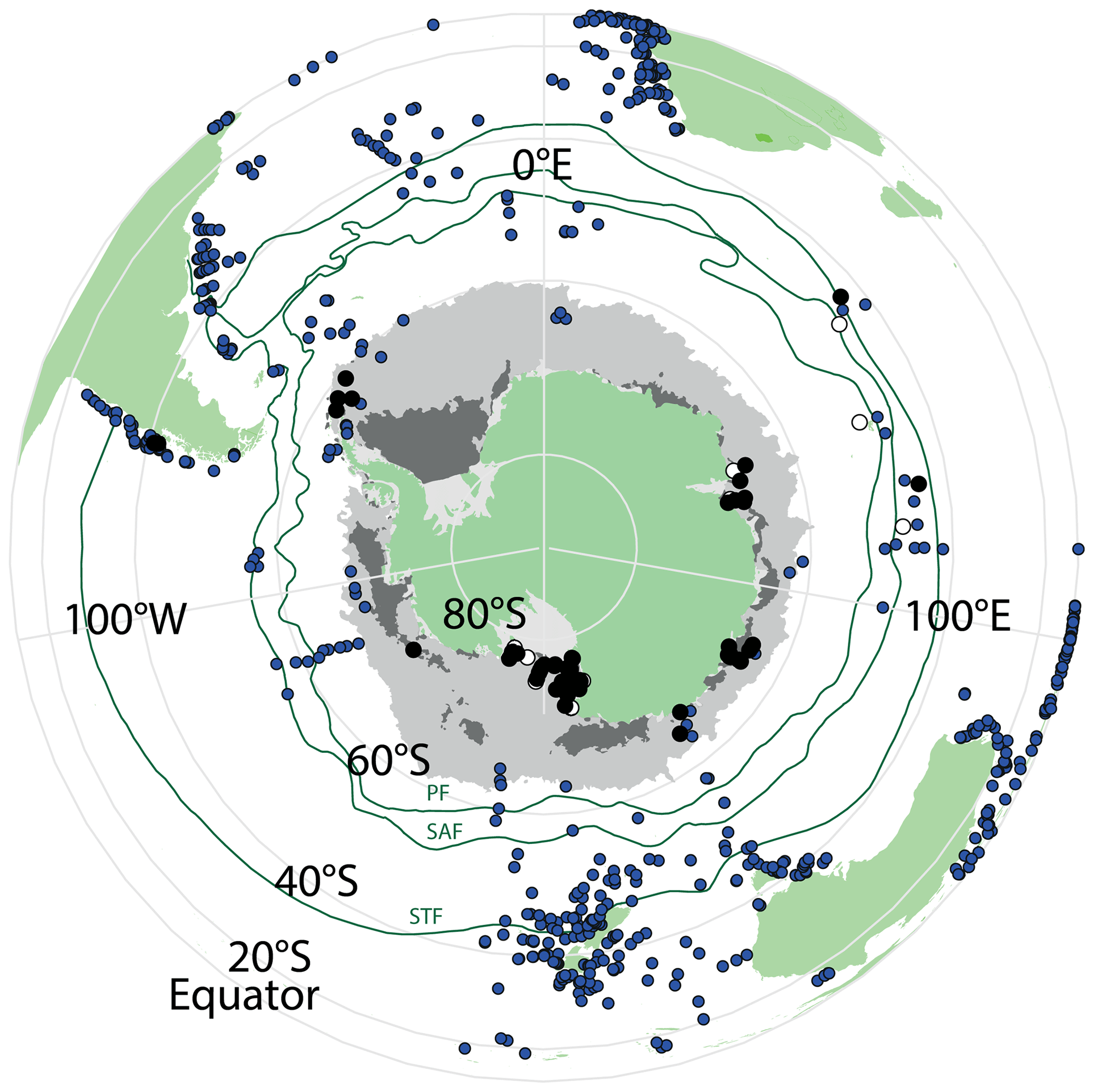
Figure 2Overview map of all available surface sediment data for the Southern Hemisphere. Blue dots represent samples that have been previously published (Marret et al., 2020), black dots are newly analysed samples from this study, and white dots are new samples that did not yield enough dinocysts to be included in further analyses. Also plotted are ACC frontal systems (dark-green lines; STF – Subtropical Front, SAF – Subantarctic Front, PF – Polar Front). Winter and summer sea ice is presented in light- and dark-grey areas, respectively, and is derived from Spreen et al. (2015–2021). Maps were produced using ggplot2 in R (Wickham, 2016).
3.2 Palynology
Samples were processed for palynological analysis following standard procedures of the Laboratory of Paleobotany and Palynology (e.g. Bijl et al., 2018b). Sediment samples were freeze-dried, crushed, and weighed before a tablet of a known amount (19 855) of Lycopodium clavatum was added to quantify dinoflagellate cyst concentrations. Samples were then treated with 30 % hydrochloric acid (HCl) and 38 % cold hydrofluoric acid to respectively dissolve carbonates and silicates. A second round of 30 % HCl treatment removed fluoric gels that might have formed before the acid sample mix was centrifuged and decanted. The (organic) residue was sieved at 250 and 10 µm, and an ultrasonic bath assisted in disaggregating organic particles. The residue was mounted on glass sides in glycerin jelly. Dinoflagellate cysts were then counted under light-transmitted light microscopy.
Where possible, specimens were identified to species level at 400× magnification. The taxonomy followed that cited in Williams et al. (2017) and the informal taxonomic descriptions in Esper and Zonneveld (2007) for some subspeciation. To facilitate the integration of our analyses with previously published datasets (Prebble et al., 2013; Marret et al., 2020), we grouped different dinocyst species the same way. This led to the following taxonomic groupings:
-
Brigantedinium spp. – Brigantedinium cariacoense, Brigantedinium simplex, and Dubridinium capitatum
-
Protoperidiniacean cysts – Lejeunecysta spp., cysts of Protoperidinium stellatum, Quinquecuspis concreta, and Votadinium calvum
-
Nematosphaeropsis labyrinthus – all Nematosphaeropsis species
-
Spiniferites hyperacanthus was combined with Spiniferites mirabilis.
-
Spiniferites bulloides was combined with Spiniferites ramosus.
-
Spiniferites belerius was combined with Spiniferites membranaceus.
-
Cysts of Protoperidinium nudum were assigned to Selenopemphix quanta.
-
All Echinidinium species were grouped.
-
Cysts of Polarella glacialis were counted but not included in the dinocyst sum.
-
Selenopemphix sp. 1 (Esper and Zonneveld, 2007) was counted separately from Selenopemphix antarctica, but these were grouped in the cluster analyses of wsi_100 and sh_655.
-
Gymnodinium spp. – all species of Gymnodinium.
In general, up to 100 (200 when possible) cysts (excluding Polarella) were counted per sample. This number captured the full diversity in our samples (see Fig. S1 in the Supplement for rarefaction analysis). As a minimal cutoff, 13 samples with total counts <25 were excluded from further analyses. In this paper, we describe dinocyst abundances qualitatively as follows: rare – <1 % of assemblage, few – 1 % to <10 %, common – 10 % to <25 %, abundant – 25 % to <50 %, and dominant – >50 %.
We excluded the cysts of Polarella glacialis in further data analyses for the following reasons: (1) ambiguity about whether the absence of Polarella in other studies is the result of its real absence or is due to other reasons. For instance, a coarser-than-10 µm mesh size often used for sieving samples could result in the loss of Polarella due to its small size. This obscures the presentation of biogeographic patterns for this species. (2) The short stratigraphic range of the species (a few hundred years in the samples from both the Ross Sea and Wilkes Land; Francesca Sangiorgi, personal observation, 2022, and Julian Hartman, personal communication, 2022, respectively) in the cores analysed so far could imply that its presence in the sediment is linked to preservation exclusively in relatively freshly deposited samples. It remains possible that Polarella abundance can be used as an indicator of sea ice if found in older sediments. With the existing knowledge, the potential of Polarella in paleoreconstructions is very limited. (3) This species is often the dominant taxon in modern samples but is absent in older samples. Since our analyses are based on percent abundance, including Polarella dilutes the percent abundance of the other taxa in the modern dataset, thereby skewing the comparison with older samples that lack Polarella. Since this study is intended to improve dinocyst-assemblage-based tools for paleoreconstructions, adding a modern cyst species that has no stratigraphic record does not improve this tool. The Polarella counts are available in the dataset on GitHub (Bijl, 2022) but are not included in relative-abundance calculations for the rest of this paper.
3.3 Datasets
To evaluate regional biogeographic consistency in ice-proximal assemblages, we created a data subset containing only sample locations with sea ice in the overlying waters. For this, we used modern modelling data and the criterion of Antarctic winter (June, July, August; JJA) sea-ice presence >0 (see Sect. 3.5 below). This data subset (wsi_100) contains 100 samples. We then added all new samples (Table 2) to the Southern Hemisphere samples of the latest existing global compilation of dinocyst surface sediments (Marret et al., 2020). This yields 655 samples in total (dataset sh_655).
Data from this paper are stored at GitHub (Bijl, 2022). The environmental data corresponding to the locations of wsi_100 and sh_655 are obtained from the Nucleus for European Modelling of the Ocean (NEMO; Madec and the NEMO team, 2008) ocean model, which is coupled to the MEDUSA-2.0 biogeochemical model (Yool et al., 2013), following the approach detailed in Sect. 3.5.
3.4 Cluster analyses
Cluster analysis of surface samples allowed us to explore spatial relationships between dinocyst assemblages and surface oceanographic conditions. These relationships in the modern day can be used to infer paleoceanographic conditions from fossil assemblages. Following the method of Prebble et al. (2013), we performed k-means cluster analyses on the relative abundance of dinocyst species for the two datasets. We ran 100 replicates for each cluster solution and chose the most stable clustering. The evaluation of the clustering of wsi_100 and sh_655 can be found in Figs. S2 and S3 in the Supplement. All analyses were done in R using the package DBSCAN (Hahsler et al., 2019).
3.5 Surface oceanographic parameters: surface versus transport data – particle tracking
To identify environmental conditions associated with the different clusters, we analysed SST (∘C), sea-ice presence (from 0–1, the fraction of grid cell that is sea-ice covered), salinity (psu), and nitrate (mmol m−3) and silicate (mmol m−3) in the surface waters at the location of the surface sediment samples. For this, we made use of the ORCA0083-N06 output from the NEMO ocean model (Madec and the NEMO team, 2008), which is coupled to the MEDUSA-2.0 biogeochemical model (Yool et al., 2013). We note that the density of environmental observations at high latitudes is low, and as such, the verification of the model output comes with an unknown degree of uncertainty. To evaluate the impact of particle transport, we compared the conditions in the overlying surface water to those of modelled backtracked surface water locations. The NEMO model provides a global three-dimensional flow field with 5-daily output and has horizontal resolution with 75 unevenly distributed vertical layers, properly reflecting the transport of Lagrangian particles by mesoscale and sub-mesoscale eddies (Nooteboom et al., 2020; Qin et al., 2014). In the first run, we recorded the surface water conditions of the overlying surface sediment locations every 3 d from 3 January 2000 until 30 December 2003. In the second run, we released virtual particles every 3 d for 4 years (from 3 January 2000 until 30 December 2003, using the OceanParcels Lagrangian simulator; Lange and van Sebille, 2017; Delandmeter and van Sebille, 2019) at the sediment surface location and backtracked them to the ocean surface using a 25 m d−1 sinking speed. This sinking speed is faster than the sinking of individual dinoflagellate cysts, as we assume some degree of particle aggregation (Nooteboom et al., 2019).
The southern boundary of the NEMO model set-up was at 77∘ S. As a result we had to relocate 11 samples that were originally located more southward to a latitude of 76.9∘ S for the model run (Table 2), assuming minimal effects on environmental and transport conditions. Similarly, nine sample locations were too close to land and, due to the model resolution, appeared to be on land in the model. Thus, their location was adjusted (Table 2) to the nearest ocean site by minimally shifting the latitude and/or longitude.
4.1 New Southern Hemisphere surface samples
The 66 newly analysed productive samples contain 24 different species (Fig. 3). Although we counted Selenopemphix antarctica and Selenopemphix sp. 1 (after Esper and Zonneveld, 2007) separately, the two species were not counted separately in previously published datasets (most of the data simply refer to Selenopemphix antarctica). In our cluster analysis, the two species are hence combined as Selenopemphix antarctica. All new samples from Antarctic-proximal sites are dominated by heterotrophic peridinioid (P) cysts (Fig. 3). The most Equatorward new samples (Fig. 3b, i) show abundant to dominant Brigantedinium spp., Impagidinium spp., Nematosphaeropsis labyrinthus, and Spiniferites spp. Typical ice-proximal species S. antarctica and Nucicla umbiliphora (e.g. Hartman et al., 2018) are rare or absent.
In the samples from the Weddell Sea (Fig. 3b, ii), Islandinium minutum is dominant, with very low contributions from Selenopemphix antarctica, Brigantedinium spp., or Impagidinium pallidum. The samples from Prydz Bay (Fig. 3b, iii) have a rather diverse assemblage with abundant Selenopemphix antarctica and common Selenopemphix sp.1, Nucicla umbiliphora, Islandinium minutum, and Brigantedinium spp. In the sample further north and outside the bay (ANT29_P3_03), Impagidinium pallidum dominates, with common Operculodinium centrocarpum. In the samples from the Sabrina Coast (Fig. 3b, iv), Selenopemphix antarctica sp. 1 is abundant, with rare to few Selenopemphix sp.1, Nucicla umbiliphora, and Islandinium minutum. A striking distinction can be made between samples from the Sabrina Coast, with one part having abundant Brigantedinium spp. and the other part having abundant Impagidinium pallidum (>30 %), common Operculodinium centrocarpum, and few Pyxidinopsis reticulata and Spiniferites mirabilis. Most of the Ross Sea samples contain an assemblage that is quite uniform (Fig. 3b, v), with dominant Selenopemphix antarctica sp. 2 and/or Nucicla umbiliphora. In most samples, one of the species is clearly dominant. Selenopemphix antarctica, Islandinium minutum, Brigantedinium spp., and Operculodinium centrocarpum are rare. In one sample located outside of the Ross Sea (ANTA02_AV43), Brigantedinium spp. dominate, with common Impagidinium pallidum and Selenopemphix antarctica.
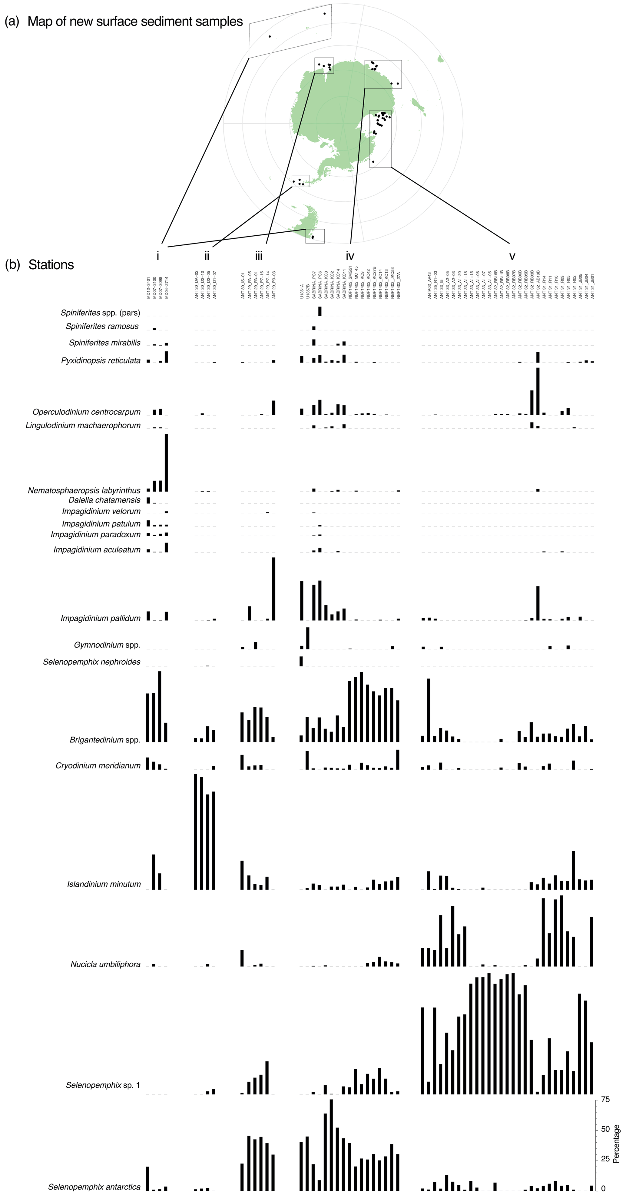
Figure 3Overview of new counted samples. (a) Map of locations of the new samples. Map was produced using ggplot2 in R (Wickham, 2016). (b) Dinocyst assemblages and absolute abundances (in cysts g−1 dry weight) for the new samples from the subantarctic or subtropical zone (i), the Antarctic Peninsula (ii), Prydz Bay (iii), the Sabrina or Wilkes Coast (iv), and the Ross Sea (v).
4.2 Clustering of the wsi_100 dataset: the Antarctic proximal sites
K-means clustering of the dinocyst assemblages in the surface sediment samples allows grouping of samples with similar dinocyst assemblages. The most stable solution for the wsi_100 dataset has five clusters (Figs. 4, S2 in the Supplement).
Cluster 1 (n=41) is dominated by Selenopemphix antarctica, with few Brigantedinium spp., Operculodinium centrocarpum, Nucicla umbiliphora, Cryodinium meridianum, and Islandinium minutum. Most samples are from the Ross Sea, and others come from along the Sabrina Coast and from West Antarctica (Fig. 4b, dark blue).
Cluster 2 (n=9) consists of nine samples and is strongly dominated by Islandinium minutum (Fig. 4a), making up almost 100 % of the average assemblage in this cluster. Only very few other species appear in this cluster, most often Brigantedinium spp. and Selenopemphix antarctica. Samples in this cluster are located in the Weddell Sea (Fig. 4b, blue).
Cluster 3 (n=13) has samples dominated by Brigantedinium spp. Other species, such as Selenopemphix antarctica, Cryodinium meridianum, Impagidinium pallidum, and Islandinium minutum, are rare. Except for one sample in the Ross Sea, Cluster 3 samples are located the furthest away from the Antarctic continent and north of 70∘ S, mainly appearing in the Pacific Ocean sector (Fig. 4b, green).
Cluster 4 (n=8) has abundant Impagidinium pallidum; common Selenopemphix antarctica; and few Brigantedinium spp., Operculodinium centrocarpum, and Pyxidinopsis reticulata. Samples from this cluster appear everywhere around Antarctica, with no clear restrictions or affinities (Fig. 4b, bright green). They are located within the Ross and Weddell seas but also further away from the Antarctic continent.
Cluster 5 (n=29) has abundant to dominant Selenopemphix antarctica. Brigantedinium spp. is common, as are Nucicla umbiliphora, Cryodinium meridianum, and Islandinium minutum. Samples in this cluster are located in the Ross Sea, Prydz Bay, and along the Sabrina Coast, mostly close to the coast (Fig. 4b, yellow).
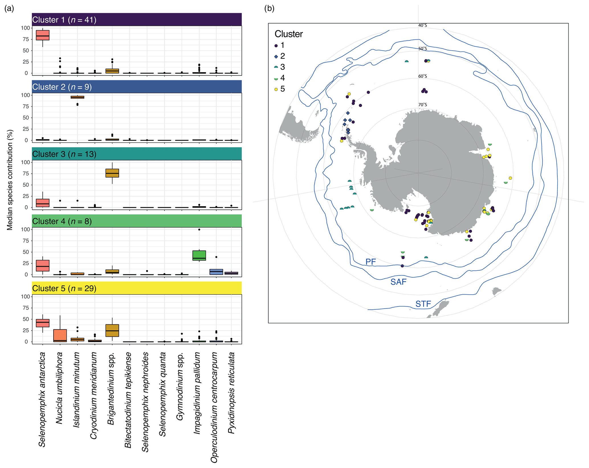
Figure 4Five-cluster solution for the wsi_100 dataset (considering all sample locations that experience surface winter (JJA) sea ice). (a) The dinocyst assemblages for each cluster (showing only the main 12 dinocyst species). Horizontal black line depicts the median, the coloured box depicts the 25 % and 75 % quantiles, and the whiskers depict the 95 % confidence interval. (b) Locations of samples colour-coded by cluster. Also plotted are frontal systems (blue lines; STF – Subtropical Front, SAF – Subantarctic Front, PF – Polar Front). Map was produced using ggplot2 in R (Wickham, 2016).
4.3 Clustering of the sh_655 dataset
The nine-cluster result of our k-means cluster analyses offers the most stable solution for the sh_655 dataset (Figs. 5, S3 in the Supplement). Below is the median dinocyst assemblage for each cluster.
In the Sant cluster (n=64), Selenopemphix antarctica dominates (Fig. 5a). Nucicla umbiliphora, Islandinium minutum, Cryodinium meridianum, and Brigantedinium spp. are common. Impagidinium pallidum and Operculodinium centrocarpum are rare. All 64 samples in this cluster are located near the Antarctic continent, such as in the Ross Sea, offshore the Sabrina Coast, and in Prydz Bay (Fig. 5b).
In the Imin cluster (n=9), dinocyst assemblages are strongly dominated by Islandinium minutum (Fig. 5a). Other species such as Brigantedinium spp. are rare. Although only very few samples (9) belong to this cluster, all are located in the Weddell Sea (Fig. 5b). These samples consistently cluster separately from the other samples in all cluster solutions (see Supplement). This cluster is identical to Cluster 2 in the wsi_100 dataset (Fig. 4).
The high-Brig cluster (n=86) is dominated by Brigantedinium spp. The assemblages are quite diverse, with few Selenopemphix quanta, various Impagidinium species, Nematosphaeropsis labyrinthus, Operculodinium centrocarpum, and Spiniferites species.
In the Nlab cluster (n=72), Nematosphaeropsis labyrinthus is abundant, with common Brigantedinium spp. Several other species, such as Impagidinium spp., Selenopemphix quanta, Selenopemphix nephroides, Operculodinium centrocarpum, Pyxidinopsis reticulata, Dalella chathamensis, and Spiniferites mirabilis, occur in low abundance. Samples are located between 40 and 60∘ S, most prominently south(west) of Tasmania and New Zealand, but also in the Indian Ocean and along the South American west coast.
In the low-Brig cluster (n=120), Brigantedinium spp. is common. Samples also contain few to common Operculodinium centrocarpum, Nematosphaeropsis labyrinthus, Impagidinium, and Spiniferites species, as well as Selenopemphix quanta and Selenopemphix nephroides. Other P cysts such as Selenopemphix antarctica, Nucicla umbiliphora, Islandinium minutum, and Cryodinium meridianum are rare. The sample locations have a wide geographic spread, but many are located around New Zealand (closer to the coast than samples from other clusters), south of Australia and around Tasmania (but in low numbers), in the mid-latitudes along the west coast of Africa, and along the west coast of South America. Samples can occasionally be found in the open ocean, for example the Indian Ocean or close to Antarctica.
In the low-Ocean cluster (n=115), no single species clearly dominates the assemblage, yet O. centrocarpum is common to abundant. Samples in this cluster are diverse. Samples contain few Brigantedinium spp., while other species have strongly variable abundance, such as Impagidinium pallidum, other Impagidinium species, Nematosphaeropsis labyrinthus, and Spiniferites spp. The geographic distribution of samples within this cluster is scattered; samples are from the Ross Sea and all along ice-proximal sites around Antarctica but also from middle and low latitudes, coastal areas, and open-ocean conditions. No clear geographical distribution is apparent.
In the Iacu cluster (n=58), Impagidinium aculeatum is abundant. Samples also contain few other Impagidinium species, Nematosphaeropsis labyrinthus, Operculodinium centrocarpum, and Brigantedinium and Spiniferites species. The samples of this cluster are mostly found between 40 and 20∘ S, although some samples are located even closer to the Equator (in the Atlantic Ocean).
The high-Ocean cluster (n=72) is dominated by Operculodinium centrocarpum, with few Brigantedinium spp., Nematosphaeropsis labyrinthus, Spiniferites mirabilis, and Spiniferites spp. Many other species occur in low abundance. Most samples of this cluster can be found close to the continental coasts of South Africa, Australia, and South America.
In the Spin cluster (n=59), Spiniferites species are abundant, with few Brigantedinium spp., Pyxidinopsis reticulata, Impagidinium species (I. aculeatum, I. patulum, and I. sphaericum) and Selenopemphix quanta. Most samples are located along the northwestern coast of Australia and in the low latitudes in the eastern Indian Ocean.
4.4 Comparison between clusters and environmental parameters
4.4.1 wsi_100: directly overlying water
Overall, the differences in oceanographic conditions are relatively small when considering the samples from the Antarctic proximal sites: nutrients are high overall, winter sea-ice presence is almost 100 %, and sea surface temperature is low (average −1.5 ∘C); however, some differences between the clusters can be identified (Fig. 6). Salinity is generally between 33.6 and 34 psu in samples from all clusters, except from Cluster 2, which has a lower median of 32.3 psu. Cluster 3 includes samples within the largest SST range (−1.4–0.2 ∘C; Fig. 6) and with the lowest sea-ice presence (median <0.7) compared to the other clusters. Clusters 1, 4, and 5 have overall very similar conditions. This means that the common Impagidinium pallidum in samples from Cluster 4 cannot be directly associated with any environmental parameters considered here.
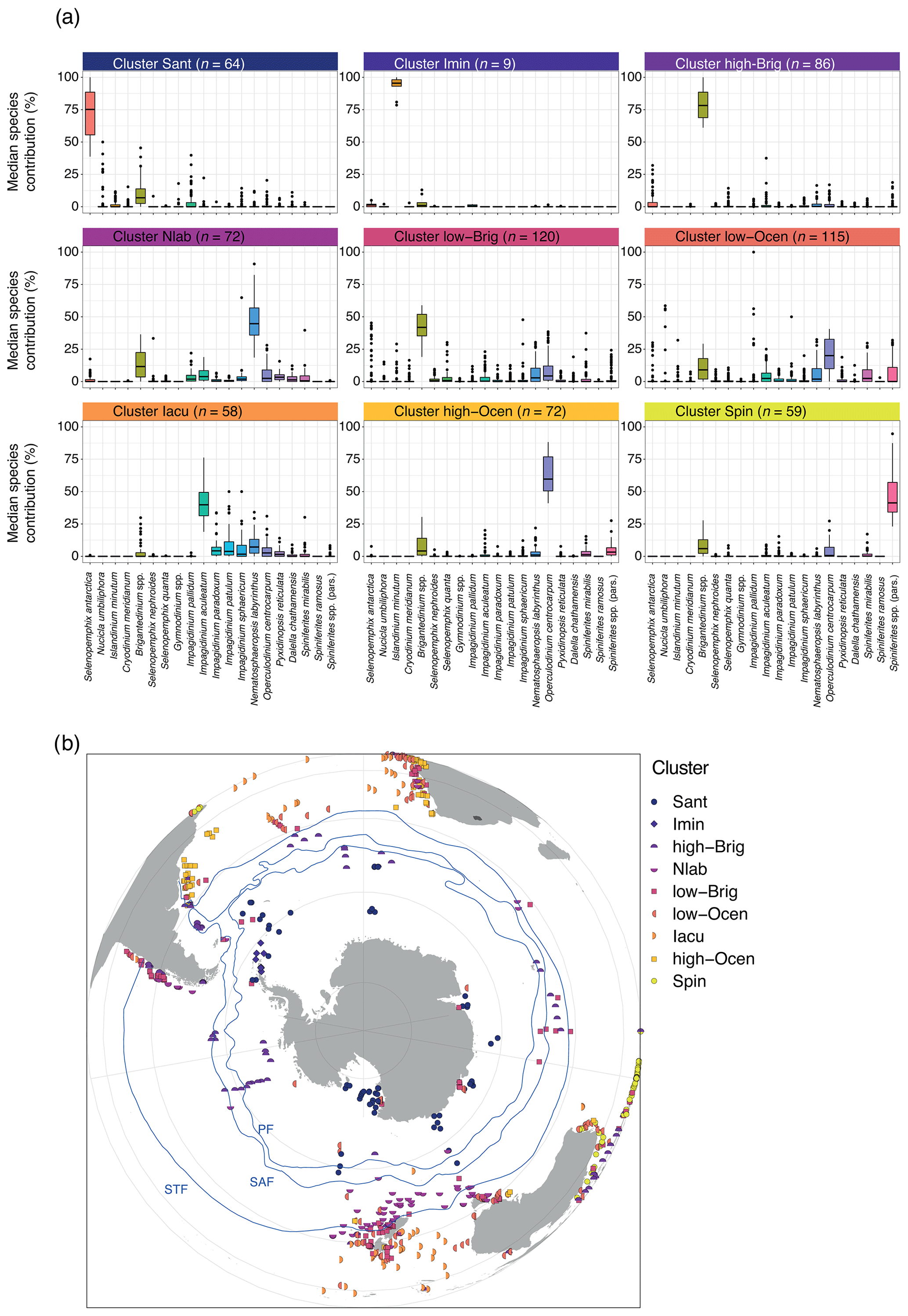
Figure 5Nine-cluster solution for the sh_655 dataset. (a) The dinocyst assemblages for each cluster (showing only the main 20 dinocyst species). Line, box, and whiskers as in Fig. 3. (b) Locations of samples colour-coded by different clusters and frontal systems (blue lines; STF – Subtropical Front, SAF – Subantarctic Front, PF – Polar Front). Map was produced using ggplot2 in R (Wickham, 2016).
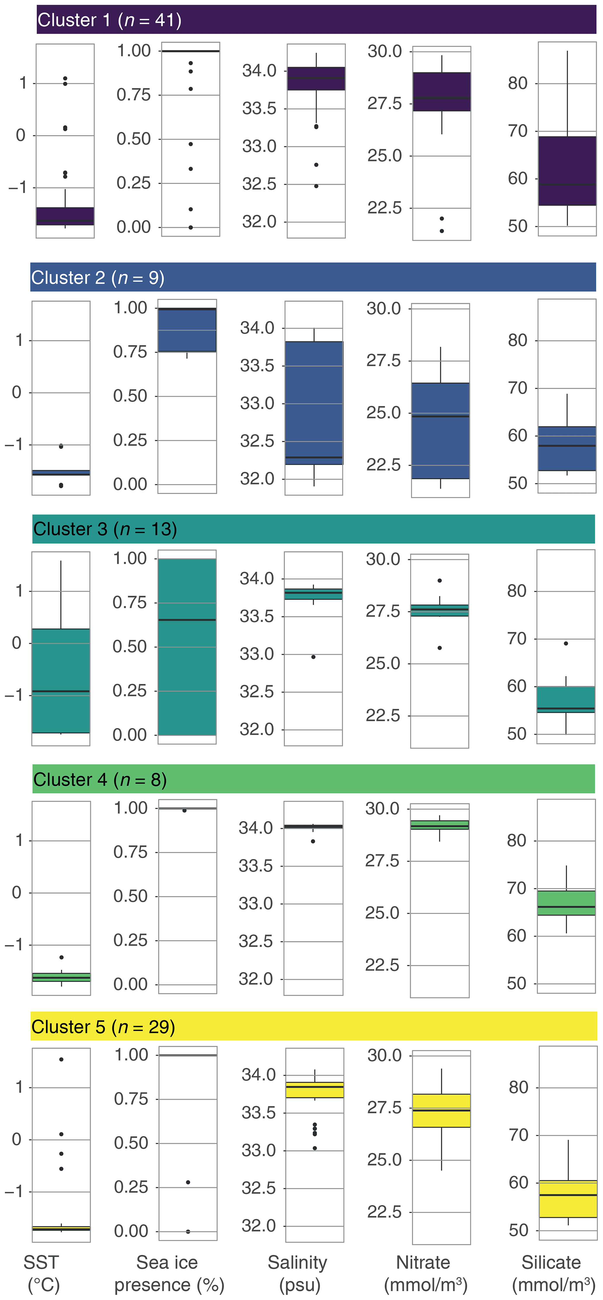
Figure 6Environmental parameters for the five-cluster solution for the wsi_100 dataset. The median (black line) of all observations per cluster (1–5), with the 25 % and 75 % quantiles depicted by the box and the whiskers depicting the 95 % confidence interval. Single points represent outliers.
4.4.2 sh_655 – assessing the effect of lateral transport on environmental affinities
To better attribute environmental parameters to the clusters in sh_655, we compare the overlying surface water conditions of each location with that of the modelled lateral particle (dinocyst) transport area due to ocean currents. Taking lateral transport into account, the source region for particles (dinocysts) is, for some samples, non-randomly offset from the directly overlying water. In the Southern Ocean south of the Subtropical Front, most transport is zonal and not meridional because of the prevailing zonal direction of currents. Regardless of their assigned cluster, all samples that are located between 40 and 60∘ S have a westward-displaced surface water source region (Fig. 7). For the Imin cluster, the source regions from the lateral transport are confined to the Weddell Sea. For the Sant cluster, the source region of samples in the Ross Sea is not displaced much when lateral transport is accounted for. Dinocysts in the samples from the Sabrina Coast and Prydz Bay originated slightly more eastwards. In general, for the Iacu cluster, the source regions are large but do not show a clear bias to latitudinal or longitudinal transport. These source regions reflect ocean-current-dictated provincialism (Fig. 7), as recently indicated by similar particle trace experiments (Nooteboom et al., 2022).
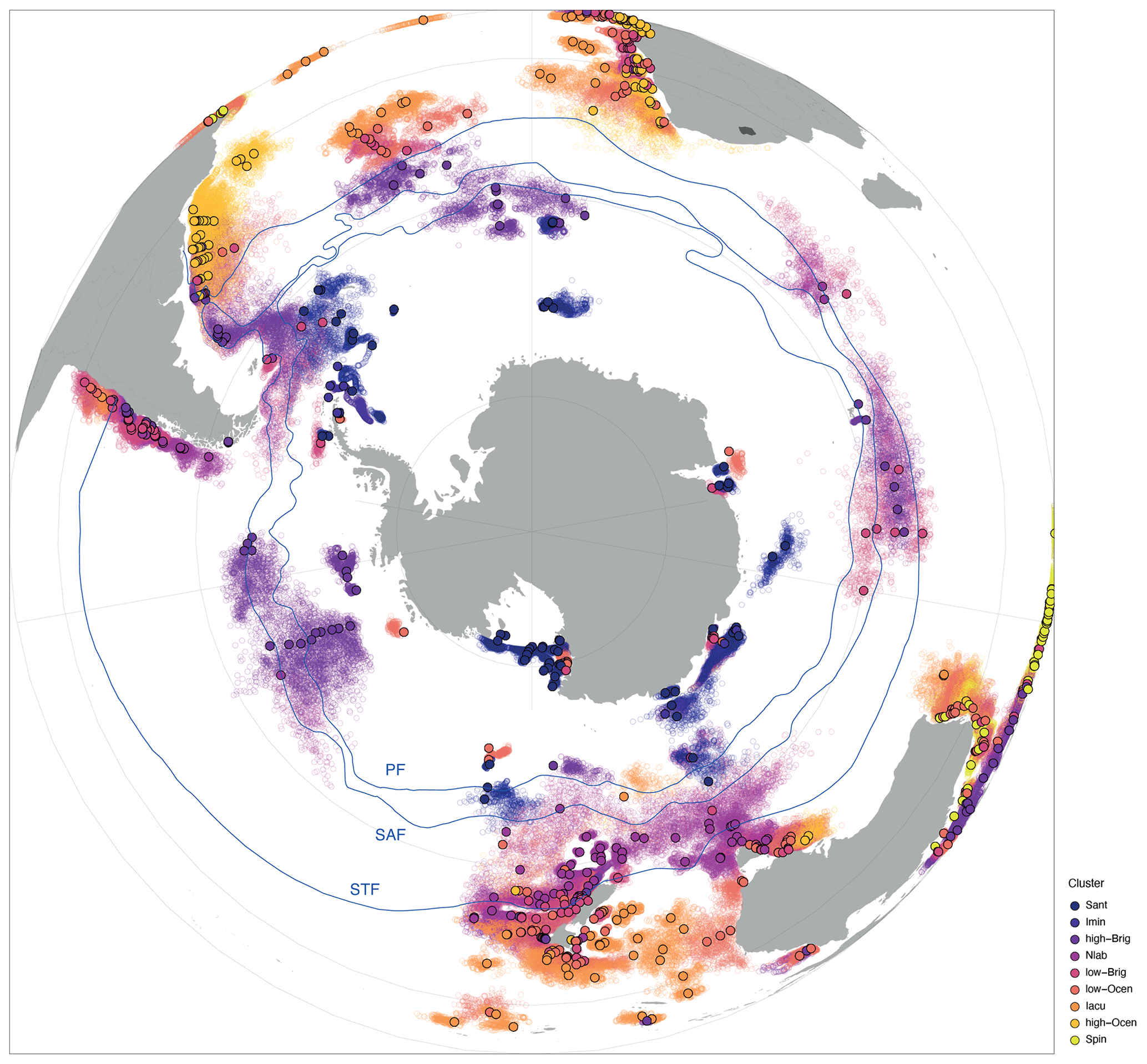
Figure 7Location and source regions of samples. Overview map of sample locations (filled dots) colour-coded by cluster with modelled surface ocean origin (open dots). Also plotted are frontal systems (blue lines; STF – Subtropical Front, SAF – Subantarctic Front, PF – Polar Front). Map was produced using ggplot2 in R (Wickham, 2016).
We compare the differences in oceanographic conditions in the median overlying surface water for each cluster in the sh_655 dataset. This can be further compared to the median conditions of the wider region after taking lateral transport into account (Fig. 8). Most clusters have distinct differences in the oceanographic conditions of the directly overlying water. The differences between the oceanographic conditions in the overlying water and the lateral transport region are, overall, small for most clusters and parameters, but some peculiarities do appear.
In the Sant cluster, there are hardly any differences between the directly overlying water and the lateral transport area. The average SST is −1.7 ∘C, and the median sea-ice presence is at 100 %. Here, the transport data show a much larger range (below 50 %) than the overlying data (below 75 %). Salinity is around 33.8 psu, and nitrate and silicate concentrations are quite high (around 27.5 and 56–57 mmol m−3, respectively).
In the Imin cluster, the average sea surface temperature for the overlying water is around −1.6 ∘C, and sea-ice presence is almost at 100 %. In the transport data, SST is around −1.7 ∘C, and sea-ice presence is 100 %. There are more striking differences between overlying and transport data in terms of salinity, nitrate, and silicate concentrations. For salinity, the overlying data show an average of around 32.3 psu with a quite large range, whereas the transported data show a much more constrained value around 33.9 psu. Nitrate and silicate concentrations in the overlying data show values around 25 and 58 mmol m−3, respectively. The transported data show values around 28 and 63 mmol m−3, respectively.
In the high-Brig cluster, overlying and transport data depict similar values. Sea surface temperature for both datasets is around 10 ∘C, sea ice is not present (only as outliers), and salinity is around 34.1 psu. Nitrate and silicate concentrations are relatively high (around 16 mmol m−3). Compared to other clusters, the range is relatively large.
In the Nlab cluster, the average sea surface temperature for both overlying and transported datasets is around 11–12 ∘C, and sea ice is not present, except in two samples. Salinity is around 34.4 psu. Nitrate concentrations are around 15 mmol m−3, and silicate concentrations are around 12 mmol m−3.
In the low-Brig cluster, the average sea surface temperature for both datasets is around 15 ∘C. Sea ice is not present, and salinity is around 34.5 psu. Nitrate and silicate concentrations are rather low (just above 10 mmol m−3 and below 5 mmol m−3, respectively).
In the low-Ocean cluster, overlying and transport data depict similar values. The average sea surface temperature for both data is around 18 ∘C, sea ice is not present, and salinity is around 35.4 psu. Nitrate and silicate concentrations are very low (<5 mmol m−3).
For the Iacu cluster, overlying and transport data are again almost identical. Sea surface temperature for both datasets is around 22.5 ∘C, and sea ice is not present. Salinity is around 35.5 psu, and nitrate and silicate concentrations are very low (<2 mmol mmol−1 m−3). The range in this cluster is very small.
In the high-Ocean cluster, the average sea surface temperature for both data is around 22 ∘C. Sea ice is not present, and salinity is around 35.5 psu. Nitrate and silicate concentrations are very low (<2 mmol m−3). The range in this cluster is relatively narrow for all parameters.
In the Spin cluster, the average sea surface temperature for both data is around 29 ∘C. Sea ice is not present, and salinity is just below 34 psu. Nitrate and silicate concentrations are exceptionally low (below 0.1 and 1 mmol m−3, respectively). The range in this cluster is very narrow for all parameters.
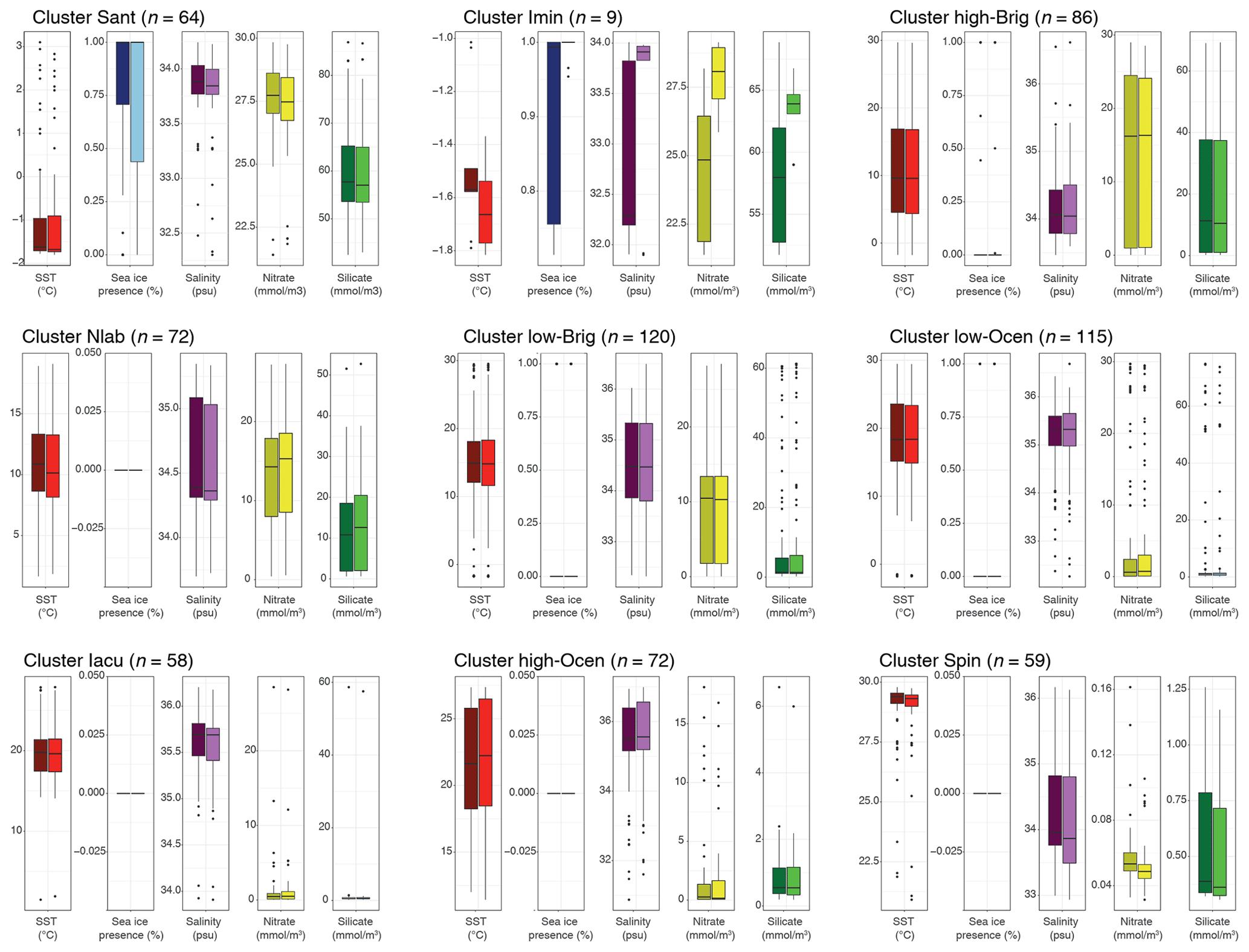
Figure 8Comparison of environmental parameters for the nine-cluster solution in the SH_655 dataset. For each cluster (Fig. 5), we compare the environmental parameters SST (red), sea-ice presence (blue), salinity (purple), nitrate (yellow), and silicate (green) of the directly overlying surface waters (left-side bar, darker fill) to those resulting from the particle transport (right-side bar, lighter fill). Black line, box, and whiskers as in Fig. 6.
5.1 Dynamics at ice-proximal sites: dinocysts as sea-ice proxy
The better representation of Antarctic ice-proximal sites in our new dataset allows us to further examine Antarctic dinocyst assemblages and associated environmental dynamics, which will help constrain paleoreconstructions. The dominance of Islandinium minutum in Weddell Sea locations is very striking (Figs. 3, 4). In the wsi_100 dataset, nine samples with high I. minutum percentages form their own cluster (Fig. 4). The cluster persists when the entire sh_655 dataset is considered (Fig. 5). This suggests that regionally unique environmental conditions strongly favour the presence of I. minutum. The source region for these samples can be placed in the Weddell Sea, suggesting that I minutum may be transported from the Weddell Sea towards the tip of the Antarctic Peninsula along with the icebergs (Iceberg Alley; Fig. 7). The low salinities of the surface waters overlying Imin cluster samples further suggest the major influence of icebergs and associated melting, as the values are the lowest of all clusters (Fig. 6; also in the sh_655 dataset, Figs. 8, 9). It seems that I. minutum dominates the assemblage in low and/or seasonally variable salinity and can thus thrive under these conditions, outcompeting other species. Other conditions such as SST, sea-ice presence, and nutrient concentrations, although slightly lower than in the other clusters, should still be high enough to promote blooms of primary productivity. As icebergs and mixing deliver enough micronutrients, there is no (local) iron limitation expected. Hence, we suggest that a high abundance or dominance of I. minutum represents strongly changing and/or relatively low salinity due to the influence of melt water in conditions otherwise typical for ice-proximal sites. Low salinity signals might also appear to be very locally restricted or punctuated in regions of high sea-ice presence, thus explaining the sparse occurrences of I. minutum in other clusters (Fig. 4).
Apart from this, there are no clear regional differences in the dinocyst abundance (Fig. 4) or clustering of the wsi_100 dataset (Fig. 6). Merging of both Selenopemphix antarctica varieties in the wsi_100 dataset limits a better delineation of the clusters (Fig. 4). Two clusters are dominated by (varying contributions of) S. antarctica (Clusters 1 and 5). Taking our newly counted samples into account, in which we separate S. antarctica into two varieties (Fig. 3), Cluster 5 mostly consists of Selenopemphix sp. 1. Also, S. antarctica dominates an assemblage alone, whereas Selenopemphix sp. 1 occurs with Nucicla umbiliphora (Figs. 3, 4). Yet, no clear geographic or environmental component can explain this difference (Figs. 3, 4, 6). If at all, one could argue that Selenopemphix sp. 1 and N. umbiliphora occur closer to the coast in the Ross Sea (Fig. 4). This might indicate that S. antarctica is more closely associated with polynya conditions. Yet, there is no polynya vs. closer-to-coast gradient visible in the environmental parameters (Fig. 6). Hence, it remains difficult to attribute environmental conditions to the separate clustering. A better distinction of S. antarctica varieties might help to further constrain the differences, although the distinction of S. antarctica into subspecies itself remains uncertain.
Despite this, a continuous sea-ice presence in these two clusters argues for a high sea-ice affinity of S. antarctica and of N. umbiliphora. This suggests that the species live either directly at the sea-ice edge or in polynyas dependent on sea-ice-driven conditions. Here, a short growth season in which micro- and macronutrients become available in an essentially unlimited amount (Swalethorp et al., 2019) fuels phytoplankton growth, allowing these heterotrophic dinoflagellate species to thrive.
Clusters 3 and 4 include the locations furthest away from the Antarctic continent and display a dominance of Brigantedinium spp. and Impagidinium pallidum but with lower numbers of S. antarctica (and N. umbiliphora) (Fig. 4). For Cluster 3, larger ranges for SST and sea-ice presence (Fig. 6) can be translated to seasonal (winter) sea-ice presence and (relatively longer) ice-free summers. We interpret this as a region where the sea-ice season is no longer the sole oceanographic factor influencing productivity. The geographic range and high nutrient concentrations (nitrate and, by inference, silicate) indicate that these locations are influenced by strong vertical mixing delivering (micro- and) macro-nutrients to the surface ocean.
This opens the question as to when low numbers of S. antarctica (or N. umbiliphora) should be considered to be a signal of low sea-ice presence or a transport signal (Nooteboom et al., 2019) in paleo-reconstructions. Again, we argue for considering the entire dinocyst assemblage. If the assemblage is dominated by species such as Brigantedinium spp., Impagidinium pallidum, or Operculodinium centrocarpum, with broad environmental niches and occurrences, we suggest considering S. antarctica and N. umbiliphora as indicators of low (seasonal) sea-ice presence. In contrast, if S. antarctica and N. umbiliphora exist in assemblages dominated by N. labyrinthus, I. aculeatum, or Spiniferites spp., we argue for a transport signal, since, in our clusters, S. antarctica and N. umbiliphora are completely absent when sea ice is absent (Figs. 5, 9 and 10). Note that this transport includes that of deep-ocean and bottom currents, which are strong in the Southern Ocean subsurface (see Nooteboom et al., 2019). Consequently, the (low) occurrences of Brigantedinium spp. in S. antarctica-dominated clusters may indicate the high tolerance of that species to sea ice and/or quick growth during (short) ice-free conditions.
5.2 SH_655 dataset: representation of Southern Hemisphere frontal zones
Compared to previous studies (e.g. Prebble et al., 2013), our study has additional surface sediment samples on both extreme ends: the warm, low-latitude end and the cold, sea-ice-influenced, polar end. As a result, our new sediment sample set better represents the full suite of Southern Hemisphere surface oceanographic conditions. From the pole towards the Equator, the clusters depict gradual warming and decreases in nitrate and silicate concentrations (Fig. 9), as seen in the modern oceanographic conditions (Fig. 1). The sea-ice-influenced zone is represented by samples from the summer and winter sea-ice edge and from regions affected by polynyas (e.g. Ross Sea and Weddell Sea) and icebergs (Antarctic Peninsula). On the warm end, the Spin cluster is a representation of warm, low-salinity but also surprisingly low-nutrient surface waters, possibly impacted by high precipitation rates (Fig. 9).
The depicted gradients in the Southern Hemisphere oceanographic conditions can be assigned to key zones in the Southern Hemisphere surface ocean, with specific oceanographic parameters (Figs. 1, 9), clearly represented by the dinocyst assemblage clusters (Fig. 5). It must be noted here that, although these clusters are characterized by one or two dominant taxa, assigning ecological affinity from assemblages should consider the full context of the dinocyst assemblage(s).
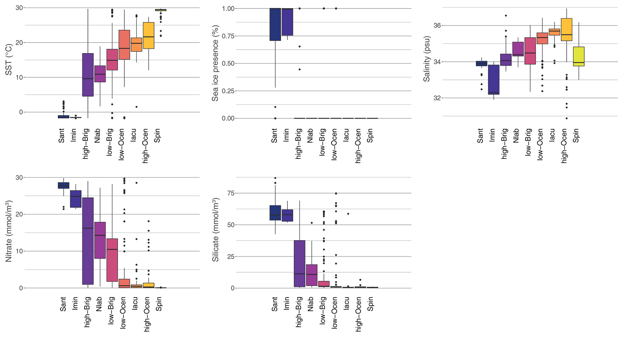
Figure 9Comparison of environmental surface conditions in different clusters for the nine-cluster solution of the sh_655 dataset. The median, 25 %–75 % quantiles, and 95 % confidence interval are indicated by the black line, boxes, and whiskers, respectively, for the environmental parameters SST (∘C), sea-ice presence (%), salinity (psu), and nitrate and silicate (mmol m−3) for each cluster, colour-coded as in Fig. 5. The environmental conditions of the directly overlying water are used here, as particle transport does not cause large differences in the environmental ranges of the clusters (see Fig. 8).
The Antarctic Zone is made up of the Sant and Imin clusters. The Antarctic Zone is clearly characterized by an abundance of P cysts, with a dominance of Selenopemphix antarctica and/or Islandinium minutum. These are the only two clusters with significant sea-ice presence and SSTs below 0 ∘C. Together with high-nutrient conditions, these two clusters clearly depict the AZ conditions of upwelling, vertical mixing, and sea-ice influence. Potentially, the high-nutrient concentrations can fuel phytoplankton growth that the dominant dinocyst species can then feed on. However, we cannot confirm if S. antarctica and/or I. minutum thrive under or at the edge of sea-ice conditions and if they could thus be used as a sea-ice proxy. The cluster also includes samples further away from the Antarctic continent (Fig. 5b), where the influence of sea ice might be limited but cold SSTs and high-nutrient conditions prevail. Thus, a quantitative estimate for past sea ice seems difficult. On the other hand, sea-ice-dominated regions like the Ross Sea, Prydz Bay, and the Sabrina Coast contain samples with high abundances of S. antarctica, suggesting that this species might at least be best adapted to sea-ice conditions. The largest difference between these two clusters can be found in their salinity range (Fig. 9). Regions within the sea-ice zone dominated by I. minutum have substantially lower salinity than those dominated by S. antarctica, and as such, the dominance of I. minutum might be taken as a low-salinity indicator in cold, sea-ice-prone environments (see Sect. 5.1).
The Subantarctic Zone is very well depicted by the Nlab cluster, dominated by N. labyrinthus. Besides that species, Brigantedinium spp., and other P or G cysts, (Impagidinium species) might be present in small numbers. The environmental parameters of this cluster are characteristic of the SAZ (Fig. 9). Although the environmental parameter profile and occurrence of many dinocyst species might indicate the transitional character of this zone, the SST range compared to other distinctly zonal clusters is quite narrow. Similarly, the STF can be very clearly identified as the northern boundary for this cluster, with a high number of N. labyrinthus occurrences (Fig. 5b), best seen around Australia, Tasmania, and New Zealand.
The clusters that best describe the conditions just north of the Subtropical Front are the Iacu cluster, with I. aculeatum being the dominant species, and the Ocean clusters, with O. centrocarpum being the dominant species. The trends of increased SST and salinity due to higher evaporation continue, and nutrient availability drops to almost zero, which is characteristic for sub-tropical conditions that are less influenced by Southern Ocean and/or ACC conditions. The environmental difference between these two clusters is difficult to discern. It seems that samples of the Ocean cluster have slightly higher nitrate (and silicate) concentrations and lower salinity (Fig. 9). For the high-Ocean cluster, this might be caused by samples of the cluster being located closer to land (Fig. 5b). This might argue for I. aculeatum needing slightly more open-ocean conditions. Considering the much narrower environmental parameter ranges in the Iacu cluster, this might indicate that I. aculeatum can dominate the assemblage in a quite specific range but is out-competed by the generalist O. centrocarpum if conditions are not optimal. Nevertheless, the drastic assemblage changes from the N. labyrinthus dominance south of the STF to the I. aculeatum or O. centrocarpum dominance north of the STF might be used to track STF positional shifts in the past. While many clusters (due to the doubled sample size – see Table 1) differ significantly from clusters identified by Prebble et al. (2013), this Nlab vs. Iacu distinction at the STF was also observed there.
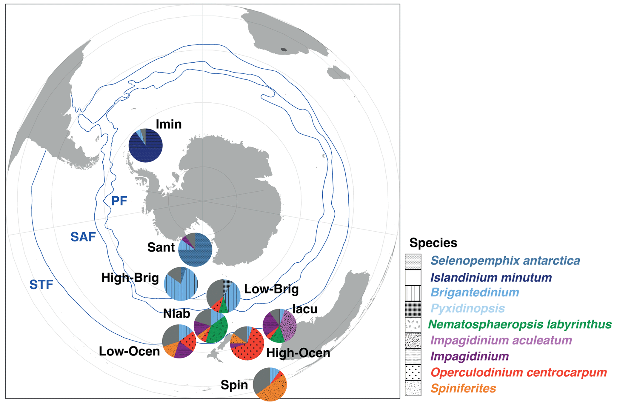
Figure 10Schematic representation of the generalized biogeographic distribution of dinocysts in Southern Ocean surface sediments. Pies represent the average assemblage composition of the nine clusters described in this paper. The position of these pies represents their typical latitudinal band of occurrence. Also plotted are the frontal systems (blue lines; STF – Subtropical Front, SAF – Subantarctic Front, PF – Polar Front). The Subantarctic Zone (SAZ) is the water mass between the STF and PF. Map was produced using ggplot2 in R (Wickham, 2016).
The cluster dominated by Spiniferites spp. appears in very low latitudes and/or locally very warm areas, such as the Australian west coast (Fig. 5), confirmed by an SST of almost 30 ∘C. What is striking is also the lower salinity of this cluster compared to that of the others.
The nine clusters are mostly clearly restricted to specific zones and regions in the Southern Hemisphere. However, there seems to be a gap remaining in the 0–8 ∘C SST range that is partly covered by either the polar clusters or the high-Brig cluster. This SST range also includes the transitional zone between 0 % and 100 % sea-ice presence. Better geographical representation of this transitional zone in surface sediment sample sets might improve the constraint of this transitional zone. On the other hand, it might be that the nature of this part of the Southern Ocean, with large-scale turbulent mixing, causes a mixed dinocyst assemblage. The large ranges of the high-Brig in terms of SST, but also in terms of nutrient concentration (Fig. 9), might best represent this dynamic environment, with Brigantedinium spp. as a more generalist species dominating the dinocyst assemblage (Fig. 5). This is also the case for the low-Brig cluster that does not show any clear oceanographic boundaries. Potentially, conditions that (temporarily) disadvantage the dominance of the expected dinocyst might allow for Brigantedinium spp. to take over and thrive. Yet, the difference between the low- and high-Brig clusters in terms of SST, but also in terms of nutrient conditions, might argue for a high Brigantedinium tolerance to cold and very dynamic Polar Frontal Zone conditions (Figs. 4, 9).
5.3 The impact of lateral transport
The size of the source regions represented in the sample stations, as visualized in Fig. 7, suggests that many surface sediment samples in the Southern Ocean are impacted by transport (see also Nooteboom et al., 2019). This is especially true for samples located within the ACC. For these locations, their source regions are consistently placed to the west, implying that the strong ACC current transports particles clockwise, eastward around Antarctica. South of the direct influence of the ACC, the source region is displaced farther towards the east due to the anticlockwise Antarctic Coastal Current. Other features that are recognizable are the Agulhas Leakage, transporting particles along the east coast of South Africa into the Atlantic Ocean, and the so-called Iceberg Alley. This area is known for a high number of icebergs drifting along the west coast and eventually out of the Weddell Sea due to the Weddell Gyre. Locations that are not directly influenced by the ACC and these smaller features do not experience such a large transport. Thus, ice-proximal and low-latitude (north of ∼ 40∘ S) sites experience relatively little transport. This can mostly be attributed to the absence of strong currents and coastal proximity.
Overall, zonal transport is much stronger than meridional transport. This does not exclude latitudinal transport (Nooteboom et al., 2019) but does limit its influence. Environmental conditions are not hugely different on a zonal scale, as they are meridional, which suggests that cysts preserved in sediments can generally be linked to overlying surface water conditions. The comparison of environmental parameters between transported particles versus those from the directly overlying water for the different clusters confirms this assumption (Fig. 8). Transport does not affect the environmental affinities of the clusters significantly. The only exception is the Imin cluster, which clearly shows the influence of transport along the Iceberg Alley. The source region of the particles is predominantly the Weddell Sea; hence, the cluster represents narrower environmental conditions (Fig. 8).
5.4 Dinocyst assemblages as a proxy for Southern Ocean frontal systems
For the regions in the Southern Ocean that were already well-represented in previous surface sediment compilations (e.g. Prebble et al., 2013), our additional samples do not require changes in earlier interpretations. Distinct dinocyst assemblages exist on either side of the frontal systems in the Southern Ocean (Fig. 10). For the Subtropical Front, the difference is mostly observed between the Nlab in the SAZ and the Ocean or Iacu north of the STF. These clusters are promising as proxies for depicting the paleolocation of the STF relative to the position of sediment records; a high abundance of Nematosphaeropsis labyrinthus means the STF was north of the study area, whereas a high abundance of Operculodinium centrocarpum or Impagidinium aculeatum indicates that the STF was south of the study area. The few samples available between the SAZ and the PF generate an unclear signal, although it seems like the assemblages transition from the abundant Nlab to high-Brig. The latter is associated with the high-nutrient conditions in the Antarctic Divergence.
This study fills a gap in the knowledge of dinocyst assemblage environmental preferences, specifically from the Antarctic ice-proximal locations. With a more solid framework to qualitatively interpret past oceanographic conditions (sea ice, nutrients, sea surface temperature, and salinity) from Southern Ocean dinocyst assemblages, (paleo)reconstructions can now be tightly constrained. The five clusters in the ice-proximal assemblages demonstrate regional heterogeneity in sea-ice ecosystems. However, Selenopemphix antarctica can be used as a sea-ice indicator, and assemblages dominated by a combination of Selenopemphix sp.1 and N. umbiliphora may also provide information on the length of the sea-ice season. Selenopemphix antarctica and Selenopemphix sp.1 need to be counted separately before further environmental interpretations and conclusions can be made.
We interpreted nine clusters in the entire Southern Hemisphere dinocyst database (n=665), which can be broadly related to various oceanographic zones in the Southern Ocean and have clear differences in their oceanographic affinities. Despite strong currents and deep basins, lateral transport of sinking particles has little effect on the relationship between surface oceanographic conditions and sedimentary assemblages. This means that, for the clusters, oceanographic conditions of the directly overlying water are a good approximation of what sedimentary plankton assemblages relate to, while lateral transport can influence sedimentary plankton assemblages at individual sites or when the results of this study are used in paleoreconstructions. From the results of the entire Southern Ocean dataset and our identified nine clusters, we identify frontal-zone-specific dinocyst assemblages, separated by the Southern Ocean fronts PF, SAF, and STF. Our results provide a solid basis for further use of dinocyst assemblages as an indicator for past oceanographic conditions in the Southern Ocean, including frontal-system locations through time.
Microscope slides are stored in the collection of the Marine Palynology and Paleoceanography group under storage code 000.000.017.533. Dinocyst data (including the counts of Polarella glacialis, sample weights, and Lycopodium counts to calculate absolute concentrations), particle trace model output, and various cluster analyses, as well as an R markdown providing the coding for the plots in this paper, are available at GitHub (https://github.com/bijlpeter83/SH655/, last access: 1 July 2022) and deposited at Zenodo (https://doi.org/10.5281/zenodo.6786422, Bijl, 2022).
The supplement related to this article is available online at: https://doi.org/10.5194/jm-42-35-2023-supplement.
PKB designed the research with FS. SH, RW, SN, and EM provided new sediment samples. LMT and SH analysed the samples. PDN contributed the Lagrangian particle trace simulations and the interpretation of the model data with IS. All the authors collaborated in analysing the results and provided input for the writing of the paper.
At least one of the (co-)authors is a member of the editorial board of Journal of Micropalaeontology. The peer-review process was guided by an independent editor, and the authors also have no other competing interests to declare.
Publisher’s note: Copernicus Publications remains neutral with regard to jurisdictional claims in published maps and institutional affiliations.
This article is part of the special issue “Advances in Antarctic chronology, paleoenvironment, and paleoclimate using microfossils: Results from recent coring campaigns”. It is not associated with a conference.
We thank Mariska Hoorweg for the analytical support in the GeoLab of the Faculty of Geosciences. We thank CNR_ISMAR, Bologna; and INGV, Pisa, Italy; and the predecessors of the International Ocean Discovery Program for providing the surface sediment samples for this project. This work was jointly supported by the National Natural Science Foundation of China (grant nos. 42030401 and 41776191). We thank the 29th and 33rd Chinese Antarctic Expedition cruise members for retrieving the sediments. The authors wish to thank the CSIRO Marine National Facility (MNF) for its support in the form of sea time on RV Investigator, support personnel, scientific equipment, and data management. All data and samples acquired on the voyage are made publicly available in accordance with the MNF Policy. The constructive and detailed reviews by Joe Prebble and one anonymous reviewer, as well as the language suggestions by the editor, significantly improved this paper.
This research has been supported by the seventh framework programme of the European Research Council (ERC Starting grant no. 802835, OceaNice to Peter Kristian Bijl).
This paper was edited by Denise K. Kulhanek and reviewed by Joe Prebble and one anonymous referee.
Adkins, J. F.: The role of deep ocean circulation in setting glacial climates, Paleoceanography, 28, 539–561, doi.org/10.1002/palo.20046, 2013.
Armand, L. K., O'Brien, P. E., and On-board Scientific Party: Interactions of the Totten Glacier with the Southern Ocean through multiple glacial cycles (IN2017-V01): Post-survey report, Research School of Earth Sciences, Australian National University, Canberra, https://doi.org/10.4225/13/5acea64c48693, 2018.
Behrens, B., Miyairi, Y., Sproson, A. D., Yamane, M., and Yokoyama, Y.: Meltwater discharge during the Holocene from the Wilkes subglacial basin revealed by beryllium isotope analysis of marine sediments, J. Quaternary Sci., 34, 603–608, https://doi.org/10.1002/jqs.3148, 2019.
Bijl, P. K.: SH655 dinocyst surface sediment database, Zenodo [data set], https://doi.org/10.5281/zenodo.6786422, 2022.
Bijl, P. K., Houben, A. J. P., Hartman, J. D., Pross, J., Salabarnada, A., Escutia, C., and Sangiorgi, F.: Paleoceanography and ice sheet variability offshore Wilkes Land, Antarctica – Part 2: Insights from Oligocene–Miocene dinoflagellate cyst assemblages, Clim. Past, 14, 1015–1033, https://doi.org/10.5194/cp-14-1015-2018, 2018a.
Bijl, P. K., Houben, A. J. P., Bruls, A., Pross, J., and Sangiorgi, F.: Stratigraphic calibration of Oligocene–Miocene organic-walled dinoflagellate cysts from offshore Wilkes Land, East Antarctica, and a zonation proposal, J. Micropalaeontol., 37, 105–138, https://doi.org/10.5194/jm-37-105-2018, 2018b.
Bromwich, D. H., Carrasco, J. F., and Stearns, C. R.: Satellite Observations of Katabatic-Wind Propagation for Great Distances across the Ross Ice Shelf, Mon. Weather Rev., 120, 1940–1949, https://doi.org/10.1175/1520-0493(1992)120<1940:sookwp>2.0.co;2, 1992.
Crosta, X., Etourneau, J., Orme, L. C., Dalaiden, Q., Campagne, P., Swingedouw, D., Goosse, H., Massé, G., Miettinen, A., McKay, R. M., Dunbar, R. B., Escutia, C., and Ikehara, M.: Multi-decadal trends in Antarctic sea-ice extent driven by ENSO–SAM over the last 2,000 years, Nat. Geosci., 14, 156–160, https://doi.org/10.1038/s41561-021-00697-1, 2021.
Delandmeter, P. and van Sebille, E.: The Parcels v2.0 Lagrangian framework: new field interpolation schemes, Geosci. Model Dev., 12, 3571–3584, https://doi.org/10.5194/gmd-12-3571-2019, 2019.
de Vernal A., Henry M., Matthiessen J., Mudie P. J., Rochon A., Boessenkool K. P., Eynaud F., Grøsfjeld K., Guiot J., Hamel D., Harland R., Head M. J., Kunz-Pirrung M., Levac E., Loucheur V., Peyron O., Pospelova V., Radi T., Turon J.-L., and Voronina E.: Dinoflagellate cyst assemblages as tracers of sea-surface conditions in the Northern North Atlantic, Arctic and sub-Arctic seas: The new “n = 67” data base and its application for quantitative palaeoceanographic reconstruction, J. Quaternary Sci., 16, 681–698, 2001.
de Vernal, A. de, Eynaud, F., Henry, M., Hillaire-Marcel, C., Londeix, L., Mangin, S., Matthiessen, J., Marret, F., Radi, T., Rochon, A., Solignac, S., and Turon, J.-L.: Reconstruction of sea-surface conditions at middle to high latitudes of the Northern Hemisphere during the Last Glacial Maximum (LGM) based on dinoflagellate cyst assemblages, Quaternary Sci. Rev., 24, 897–924, https://doi.org/10.1016/j.quascirev.2004.06.014, 2005.
de Vernal, A., de, Radi, T., Zaragosi, S., Van Nieuwenhove, N., Rochon, A., Allan, E., De Schepper, S., Eynaud, F., Head, M.J., Limoges, A., Londeix, L., Marret, F., Matthiessen, J., Penaud, A., Pospelova, V., Price, A., and Richerol, T.: Distribution of common modern dinoflagellate cyst taxa in surface sediments of the Northern Hemisphere in relation to environmental parameters: The new n=1968 database, Mar. Micropaleontol., 159, 101796, https://doi.org/10.1016/j.marmicro.2019.101796, 2020.
Esper, O. and Zonneveld, K. A. F.: The potential of organic-walled dinoflagellate cysts for the reconstruction of past sea-surface conditions in the Southern Ocean, Mar. Micropaleontol., 65, 185–212, https://doi.org/10.1016/j.marmicro.2007.07.002, 2007.
Hahsler, M., Piekenbrock, M., and Doran, D.: dbscan: Fast Density-Based Clustering with R, J. Stat. Softw., 1, 1–30, https://doi.org/10.18637/jss.v091.i01, 2019.
Harland, R. and Pudsey, C. J.: Dinoflagellate cysts from sediment traps deployed in the Bellingshausen, Weddell and Scotia seas, Antarctica, Mar. Micropaleontol., 37, 77–99, https://doi.org/10.1016/s0377-8398(99)00016-x, 1999.
Hartman, J. D., Bijl, P. K., and Sangiorgi, F.: A review of the ecological affinities of marine organic microfossils from a Holocene record offshore of Adélie Land (East Antarctica), J. Micropalaeontol., 37, 445–497, https://doi.org/10.5194/jm-37-445-2018, 2018.
Hoem, F. S., Valero, L., Evangelinos, D., Escutia, C., Duncan, B., McKay, R. M., Brinkhuis, H., Sangiorgi, F., and Bijl, P. K.: Temperate Oligocene surface ocean conditions offshore of Cape Adare, Ross Sea, Antarctica, Clim. Past, 17, 1423–1442, https://doi.org/10.5194/cp-17-1423-2021, 2021a.
Hoem, F. S., Sauermilch, I., Hou, S., Brinkhuis, H., Sangiorgi, F., and Bijl, P. K.: Late Eocene–early Miocene evolution of the southern Australian subtropical front: a marine palynological approach, J. Micropalaeontol., 40, 175–193, https://doi.org/10.5194/jm-40-175-2021, 2021b.
Houben, A. J. P., Bijl, P. K., Pross, J., Bohaty, S. M., Passchier, S., Stickley, C. E., Röhl, U., Sugisaki, S., Tauxe, L., Flierdt, T. van de, Olney, M., Sangiorgi, F., Sluijs, A., Escutia, C., Brinkhuis, H., Scientists, E. 318, Dotti, C. E., Klaus, A., Fehr, A., Williams, T., Bendle, J. A. P., Carr, S. A., Dunbar, R. B., Flores, J.-A., Gonzàlez, J. J., Hayden, T. G., Iwai, M., Jimenez-Espejo, F. J., Katsuki, K., Kong, G. S., McKay, R. M., Nakai, M., Pekar, S. F., Riesselman, C., Sakai, T., Salzmann, U., Shrivastava, P. K., Tuo, S., Welsh, K., and Yamane, M.: Reorganization of Southern Ocean Plankton Ecosystem at the Onset of Antarctic Glaciation, Science, 340, 341–344, https://doi.org/10.1126/science.1223646, 2013.
Lange, M. and van Sebille, E.: Parcels v0.9: prototyping a Lagrangian ocean analysis framework for the petascale age, Geosci. Model Dev., 10, 4175–4186, https://doi.org/10.5194/gmd-10-4175-2017, 2017.
Locarnini, A., R., Mishonov, A. V., Baranova, O. K., Boyer, T. P., Zweng, M. M., Garcia, H. E., Reagan, J. R., Seidov, D., Weathers, K., Paver, C. R., and Smolyar, I.: WORLD OCEAN ATLAS 2018, Vol. 1, Temperature, Technical Editor: Mishonov, A., NOAA Atlas NESDIS 81, 52 pp., 2018.
Madec, G. and the NEMO team: NEMO ocean engine. Note du Pôle de modélisation, Institut Pierre-Simon Laplace (IPSL), France, No. 27, ISSN No. 1288-1619, 2008.
Marret, F., Vernal, A. de, Benderra, F., and Harland, R.: Late Quaternary sea-surface conditions at DSDP Hole 594 in the southwest Pacific Ocean based on dinoflagellate cyst assemblages, J. Quaternary Sci., 16, 739–751, https://doi.org/10.1002/jqs.648, 2001.
Marret, F. and Zonneveld, K. A. F.: Atlas of modern organic-walled dinoflagellate cyst distribution, Rev. Palaeobot. Palynol., 125, 1–200, https://doi.org/10.1016/S0034-6667(02)00229-4, 2003.
Marret, F., Bradley, L., Vernal, A. de, Hardy, W., Kim, S.-Y., Mudie, P., Penaud, A., Pospelova, V., Price, A. M., Radi, T., and Rochon, A.: From bi-polar to regional distribution of modern dinoflagellate cysts, an overview of their biogeography, Mar. Micropaleontol., 159, 101753, https://doi.org/10.1016/j.marmicro.2019.101753, 2020.
Marschalek, J. W., Zurli, L., Talarico, F., van de Flierdt, T., Vermeesch, P., Carter, A., Beny, F., Bout-Roumazeilles, V., Sangiorgi, F., Hemming, S. R., Pérez, L. F., Colleoni, F., Prebble, J. G., van Peer, T. E., Perotti, M., Shevenell, A. E., Browne, I., Kulhanek, D. K., Levy, R., Harwood, D., Sullivan, N. B., Meyers, S. R., Griffith, E. M., Hillenbrand, C.-D., Gasson, E., Siegert, M. J., Keisling, B., Licht, K. J., Kuhn, G., Dodd, J. P., Boshuis, C., De Santis, L., McKay, R. M., Ash, J., Browne, I. M., Cortese, G., Dodd, J. P., Esper, O. M., Gales, J. A., Harwood, D. M., Ishino, S., Kim, S., Kim, S., Laberg, J. S., Leckie, R. M., Müller, J., Patterson, M. O., Romans, B. W., Romero, O. E., Seki, O., Singh, S. M., Cordeiro de Sousa, I. M., Sugisaki, S. T., Xiao, W., and Xiong, Z.: A large West Antarctic Ice Sheet explains early Neogene sea-level amplitude, Nature, 600, 7889, 450–455, 2021.
Marshall, J. and Speer, K.: Closure of the meridional overturning circulation through Southern Ocean upwelling, Nat. Geosci., 5, 171–180, https://doi.org/10.1038/ngeo1391, 2012.
Mitchell, B. G., Brody, E. A., Holm-Hansen, O., McClain, C., and Bishop, J.: Light limitation of phytoplankton biomass and macronutrient utilization in the Southern Ocean, Limnol. Oceanogr., 36, 1662–1677, https://doi.org/10.4319/lo.1991.36.8.1662, 1991.
Mudie, P. J., Marret, F., Mertens, K. N., Shumilovskikh, L., and Leroy, S. A. G.: Atlas of modern dinoflagellate cyst distributions in the Black Sea Corridor: from Aegean to Aral Seas, including Marmara, Black, Azov and Caspian Seas, Mar. Micropaleontol., 134, 1–152, https://doi.org/10.1016/j.marmicro.2017.05.004, 2017.
Nooteboom, P. D., Bijl, P. K., Sebille, E., Heydt, A. S., and Dijkstra, H. A.: Transport Bias by Ocean Currents in Sedimentary Microplankton Assemblages: Implications for Paleoceanographic Reconstructions, Paleoceanogr. Paleocl., 34, 1178–1194, https://doi.org/10.1029/2019pa003606, 2019.
Nooteboom, P. D., Delandmeter, P., Sebille, E. van, Bijl, P. K., Dijkstra, H. A., and von der Heydt, A. S.: Resolution dependency of sinking Lagrangian particles in ocean general circulation models, Plos One, 15, e0238650, https://doi.org/10.1371/journal.pone.0238650, 2020.
Nooteboom, P. D., Bijl, P. K., Kehl, C., van Sebille, E., Ziegler, M., von der Heydt, A. S., and Dijkstra, H. A.: Sedimentary microplankton distributions are shaped by oceanographically connected areas, Earth Syst. Dynam., 13, 357–371, https://doi.org/10.5194/esd-13-357-2022, 2022.
Orsi, A. H., Whitworth, T., and Nowlin, W. D.: On the meridional extent and fronts of the Antarctic Circumpolar Current, Deep-Sea Res., 42, 641–673, https://doi.org/10.1016/0967-0637(95)00021-w, 1995.
Park, Y. H., Park, T., Kim, T. W., Lee, S. H., Hong, C. S., Lee, J. H., Rio, M. H., Pujol, M. I., Ballarotta, M., Durand, I., and Provost, C.: Observations of the Antarctic Circumpolar Current Over the Udintsev Fracture Zone, the Narrowest Choke Point in the Southern Ocean, J. Geophys. Res.-Ocean., 124, 4511–4528, https://doi.org/10.1029/2019JC015024, 2019.
Prebble, J. G., Crouch, E. M., Carter, L., Cortese, G., Bostock, H., and Neil, H.: An expanded modern dinoflagellate cyst dataset for the Southwest Pacific and Southern Hemisphere with environmental associations, Mar. Micropaleontol., 101, 33–48, https://doi.org/10.1016/j.marmicro.2013.04.004, 2013.
Prebble, J. G., Crouch, E. M., Cortese, G., Carter, L., Neil, H., and Bostock, H.: Southwest Pacific sea surface conditions during Marine Isotope Stage 11 – Results from dinoflagellate cysts, Palaeogeogr. Palaeocl., 446, 19–31, https://doi.org/10.1016/j.palaeo.2016.01.007, 2016.
Qin, X., Sebille, E. van, and Gupta, A. S.: Quantification of errors induced by temporal resolution on Lagrangian particles in an eddy-resolving model, Ocean Model., 76, 20–30, https://doi.org/10.1016/j.ocemod.2014.02.002, 2014.
Rhodes, R. H., Bertler, N. A. N., Baker, J. A., Sneed, S. B., Oerter, H., and Arrigo, K. R.: Sea ice variability and primary productivity in the Ross Sea, Antarctica, from methylsulphonate snow record, Geophys. Res. Lett., 36, 37311, https://doi.org/10.1029/2009gl037311, 2009.
Sangiorgi, F., Bijl, P. K., Passchier, S., Salzmann, U., Schouten, S., McKay, R., and Bohaty, S. M.: Southern Ocean warming and Wilkes Land ice sheet retreat during the mid-Miocene, Nat. Commun., 9, 317, https://doi.org/10.1038/s41467-017-02609-7, 2018.
Solodoch, A., Stewart, A. L., Hogg, A. M., Morrison, A. K., Kiss, A. E., Thompson, A. F., Purkey, S. G., and Cimoli, L.: How Does Antarctic Bottom Water Cross the Southern Ocean?, Geophys. Res. Lett., 49, e2021GL097211, https://doi.org/10.1029/2021GL097211, 2022.
Spreen, G., Melsheimer, C., and Malte Gerken, M.: Sea ice remote sensing, Institute of Environmental Physics, University of Bremen, Germany, https://seaice.uni-bremen.de/databrowser/ (last access: 17 December 2022). 2015–2021.
Swalethorp, R., Dinasquet, J., Logares, R., Bertilsson, S., Kjellerup, S., Krabberød, A. K., Moksnes, P.-O., Nielsen, T. G., and Riemann, L.: Microzooplankton distribution in the Amundsen Sea Polynya (Antarctica) during an extensive Phaeocystis antarctica bloom, Prog. Oceanogr., 170, 1–10, https://doi.org/10.1016/j.pocean.2018.10.008, 2019.
Talley, L.: Closure of the Global Overturning Circulation Through the Indian, Pacific, and Southern Oceans: Schematics and Transports, Oceanography, 26, 80–97, https://doi.org/10.5670/oceanog.2013.07, 2013.
Wickham, H.: ggplot2: Elegant Graphics for Data Analysis, Springer-Verlag New York, ISBN 978-3-319-24277-4, https://ggplot2.tidyverse.org (last access: 30 May 2023), 2016.
Williams, G. L., Fensome, R. A., and MacRae, R. A.: The Lentin and Williams Index of Fossil Dinoflagellates, The Lentin and Williams index of fossil dinoflagellates 2017 edition, American Association of Stratigraphic Palynologists Contributions Series, no. 48, https://doi.org/10.4095/103330, 2017.
Wilson, D. J., Bertram, R. A., Needham, E. F., van de Flierdt, T., Welsh, K. J., McKay, R. M., Mazumder, A., Riesselman, C. R., Jimenez-Espejo, F. J., and Escutia, C.: Ice loss from the East Antarctic Ice Sheet during late Pleistocene interglacials, Nature, 561, 383–386, https://doi.org/10.1038/s41586-018-0501-8, 2018.
Yool, A., Popova, E. E., and Anderson, T. R.: MEDUSA-2.0: an intermediate complexity biogeochemical model of the marine carbon cycle for climate change and ocean acidification studies, Geosci. Model Dev., 6, 1767–1811, https://doi.org/10.5194/gmd-6-1767-2013, 2013.
Zonneveld, K. A. F., Marret, F., Versteegh, G. J. M., Bogus, K., Bonnet, S., Bouimetarhan, I., Crouch, E., Vernal, A. de, Elshanawany, R., Edwards, L., Esper, O., Forke, S., Grøsfjeld, K., Henry, M., Holzwarth, U., Kielt, J.-F., Kim, S.-Y., Ladouceur, S., Ledu, D., Chen, L., Limoges, A., Londeix, L., Lu, S.-H., Mahmoud, M. S., Marino, G., Matsouka, K., Matthiessen, J., Mildenhal, D. C., Mudie, P., Neil, H. L., Pospelova, V., Qi, Y., Radi, T., Richerol, T., Rochon, A., Sangiorgi, F., Solignac, S., Turon, J.-L., Verleye, T., Wang, Y., Wang, Z., and Young, M.: Atlas of modern dinoflagellate cyst distribution based on 2405 data points, Rev. Palaeobot. Palyno., 191, 1–197, https://doi.org/10.1016/j.revpalbo.2012.08.003, 2013.