Deep learning accurately identifies fjord benthic foraminifera

Over the past several decades, there has been increasing interest in using foraminifera as environmental indicators for coastal marine environments. Foraminifera provide equally good environmental quality status assessment as compared to large invertebrates (macrofauna), which are currently used as biological quality elements. However, foraminifera offer several distinct advantages as bioindicators, including short response and generation times, a high number of individuals per small sample volume, and hard and fossilizing shells with a potential of paleoecological record. One of the major challenges in foraminifera identification is the reliance on manual morphological methods, which are not only time-consuming and error-prone but also highly dependent on the expertise of taxonomic specialists. Deep learning, a subfield of machine learning (ML), has emerged as a promising solution to this challenge, since a neural network can learn to recognize subtle differences in shell morphology that may be difficult for the human eye to distinguish. In addition, the speed and ease afforded by deep learning methods would allow experts and non-experts alike to use foraminifera more extensively in their work, thus helping to integrate the use of foraminifera in biomonitoring programs by agencies and industry. This study focuses on benthic foraminifera from several Skagerrak fjords, including Gullmar Fjord, Hakefjord, Sannäs Fjord, and Idefjord (Fig. 1a). Sediment archives from these fjords provide extensive records of past and ongoing climate and environmental changes. Fjord foraminifera mounted on microslides were imaged using a stereomicroscope (3003 images), and individual foraminifera were labeled using the Roboflow online platform (22 138 individuals). Using the labeled images, we trained a You Only Look Once (YOLO) v7 deep learning model, which demonstrates state-of-the-art speed and performance for object detection as of the time of writing. The models can distinguish among 29 species with 90.3 % and 78.8 % mean average precision in the best- and the worst-performing models, respectively. Even though the imaging and labeling was done in a short amount of time (∼ 300 h over a course of 2 months), the results show that even a relatively small dataset can be used for training a reliable deep learning species identification model.

1 Introduction

Benthic foraminifera are single-celled eukaryotes that are widely used in environmental monitoring due to their sensitivity to environmental changes (e.g., Bouchet et al., 2012; Dolven et al., 2013; Polovodova Asteman et al., 2015; Alve et al., 2019; O'Brien et al., 2021). The majority of benthic foraminifera construct calcareous or agglutinated shells; the high preservation potential of these shells, in combination with their high abundance in small sample volumes and the rapid response of benthic foraminifer populations to environmental changes, makes benthic foraminifera ideal for tracking both short- and long-term ecological shifts in modern and ancient marine environments (Alve et al., 2009). Foraminiferal distribution, diversity, and morphology can provide key insights into oceanographic conditions, including temperature, salinity, oxygen levels, and pollution (Alve, 1995; Murray, 2006). The above-mentioned qualities make these microeukaryotes useful proxies in paleoceanography and paleoclimate research and valuable bioindicators in environmental research. Over the past several decades, benthic foraminifera have been increasingly used in environmental monitoring in coastal waters and were shown to characterize environmental quality status equally well as traditional macrofaunal bioindicators (Dolven et al., 2013; Alve et al., 2019). Foraminifera have been applied to monitor pollutants such as heavy metals (e.g., Alve, 1991; Frontalini and Coccioni, 2008; Dolven et al., 2013; Polovodova Asteman et al., 2015; Boehnert et al., 2020; Lintner et al., 2021) and hydrocarbons (e.g., Morvan et al., 2004; Ernst et al., 2006; Brunner et al., 2013; Schwing et al., 2015, Frontalini et al., 2020), with their population dynamics offering insights into ecosystem health, particularly in areas experiencing stress from hypoxia or eutrophication (Bernhard and Alve, 1996; Filipsson and Nordberg, 2004).

Traditionally, the identification of foraminifera has relied on manual identification methods based on shell morphology (e.g., pore patterns, wall texture, sutures, chamber arrangement), requiring expert knowledge and significant time investment. This process involves the examination of samples under a stereomicroscope to manually pick specimens (generally < 1 mm in size, using a fine brush) and to count and classify the organisms to the lowest possible taxonomic level. Manual identification is not only slow but also prone to human error (e.g., Austen et al., 2016; Austen et al., 2018; Fenton et al., 2018), leading to potential biases and misinterpretations of results (see Hsiang et al., 2019, for discussion of rarity biases in human classifiers of planktonic foraminifera). Additionally, manual identification limits the scale of analysis, as it is difficult to process large datasets manually in a reasonable time frame, resulting in a lengthy process of data collection taking months to years depending on the size of the team involved (Hsiang et al., 2019). Given the increasing demand for high-throughput environmental monitoring data, particularly in response to pressing issues such as climate change and pollution, there is a growing need to automate the identification process of foraminifera to facilitate their use as bioindicators, as advocated by the FOBIMO protocol (Schönfeld et al., 2012).

Recent advances in machine learning (ML), particularly deep learning techniques, offer promising solutions to these challenges. Convolutional neural networks (CNNs), a class of deep learning algorithm designed to process, classify, and segment images, have revolutionized the field of image recognition (Krizhevsky et al., 2012; LeCun et al., 2015). CNNs are highly effective at learning complex patterns and features in images, making them ideal for tasks such as species identification from microscopy images. CNNs achieve this by automatically learning to detect features such as edges, textures, and shapes in images by using convolutional layers, which apply filters to the input images, creating feature maps that highlight specific visual characteristics of the objects in the image (Dumoulin and Visin, 2016). By stacking multiple convolutional layers, CNNs can learn to recognize complex patterns such as the intricate morphological details of foraminiferal shells. Unlike traditional image recognition methods, CNNs can perform feature extraction without manual pre-processing and hand-crafted features by learning features directly from the data. This allows CNNs to generalize better to new images (Castro et al., 2017), allowing more widespread deployment and application of trained models.

While CNNs are effective for image classification, many ecological studies require not only classification but also object detection. Object detection involves identifying and localizing specific objects within an image. This is particularly important in cases where multiple objects of interest (such as different species of foraminifera) may appear in the same image, and the model needs to detect and classify each object individually. The You Only Look Once (YOLO) family of models represents a state-of-the-art approach to object detection in deep learning (Redmon et al., 2015). YOLO models are known for their speed and accuracy, making them particularly well suited for real-time applications where quick detection is crucial, such as for face recognition algorithms in mobile devices and smart cameras (Chen et al., 2021; Yu et al., 2024). In the context of foraminiferal research, machine learning models like YOLO can automate the detection and classification of species, dramatically reducing the time required for analysis. Several studies have successfully applied deep learning to planktonic foraminifera (Mitra et al., 2019; Hsiang et al., 2019; Marchant et al., 2020; Karaderi et al., 2022; Ferreira-Chacua and Koeshidayatullah, 2023), but there has been comparatively limited research focused on the application of these techniques to benthic foraminifera, particularly those from fjord environments (but see Govindakutty Menon et al., 2023, deep learning for pore detection).

The Skagerrak (North Sea) and its fjords, located along the Swedish and Norwegian coastlines, are home to a rich diversity of benthic foraminifera with communities ranging from estuarine to oceanic species (Fig. 1b). The fjords represent contrasting environmental conditions, ranging from well oxygenated (Hakefjord: Watts et al., 2024; O'Brien et al., 2025) to severely hypoxic (Gullmar Fjord and Sannäs Fjord: Nordberg et al., 2000, 2017; Choquel et al., 2021) and from relatively deep (Gullmar Fjord: > 110 m) to shallow water conditions (Sannäs Fjord: 7–25 m; Nordberg et al., 2017). Despite serving as important carbon sinks (Watts et al., 2024), some of the Skagerrak fjords today experience high natural and anthropogenic pressures, including eutrophication, various industrial discharges, introduction of alien and invasive species, and climate-related changes in bottom water temperature, salinity, and oxygenation (e.g., Filipsson and Nordberg, 2004; Dolven et al., 2013; Polovodova Asteman et al., 2015; Karlsson et al., 2018; Mattsson et al., 2022; Choquel et al. 2023; O'Brien et al., 2025; McGann et al., 2025). For instance, species typical of the so-called Skagerrak–Kattegat (S–K) fauna (Cassidulina laevigata, Textularia earlandi, Bulimina marginata, Liebusella goesi, Hyalinea balthica, and Nonionellina labradorica), the opportunistic species Stainforthia fusiformis, and the non-indigenous and putatively invasive Nonionella sp. T1 are commonly used as bioindicators for monitoring environmental changes in these regions (Nordberg et al., 2000; Dolven et al., 2013; Polovodova Asteman and Schönfeld, 2015). The S–K fauna and S. fusiformis show clear responses to bottom water hypoxia, making them valuable for reconstructing past and present ecological conditions (Alve, 2003; Polovodova Asteman and Nordberg, 2013). Furthermore, the recent discovery of putatively invasive Nonionella sp. T1 in the Skagerrak has raised concerns about the shifting dynamics within the foraminiferal communities there (e.g., Polovodova Asteman and Schönfeld, 2015; Deldicq et al., 2019; Brinkmann et al., 2023; Morin et al., 2023). This species now thrives in nitrate-rich fjord sediments and may outcompete native species under severely hypoxic conditions due to its ability to respire nitrate through denitrification (Choquel et al., 2021).

With the ongoing climate change shifting climatic zones and intense marine traffic, more and more coastal settings will become a new home for alien and invasive foraminifera species, further emphasizing the need for new and more efficient monitoring methods offered by deep learning and image recognition. This study explores the application of convolutional neural networks (CNNs) and the You Only Look Once (YOLO) architecture to identify benthic foraminifera species from the Skagerrak and its fjords. Our aim is to demonstrate the feasibility of these models for performing complex morphological identification and detection of benthic foraminifera, offering a potential solution to the limitations of manual identification of benthic foraminifera and thus opening up the path towards their widespread usage as bioindicators for rapid, automated monitoring of marine coastal environments.

2 Materials and methods

2.1 Image acquisition

The dataset for this study was generated from > 70 sediment samples collected from the Skagerrak fjords, including the Gullmar Fjord, the Hakefjord, the Sannäs Fjord, and the Idefjord over the time period 2009–2023 (Figs. 1 and 2a). These fjords are located along the western coastline of Sweden and are known for their ecological diversity and dynamic marine environments.

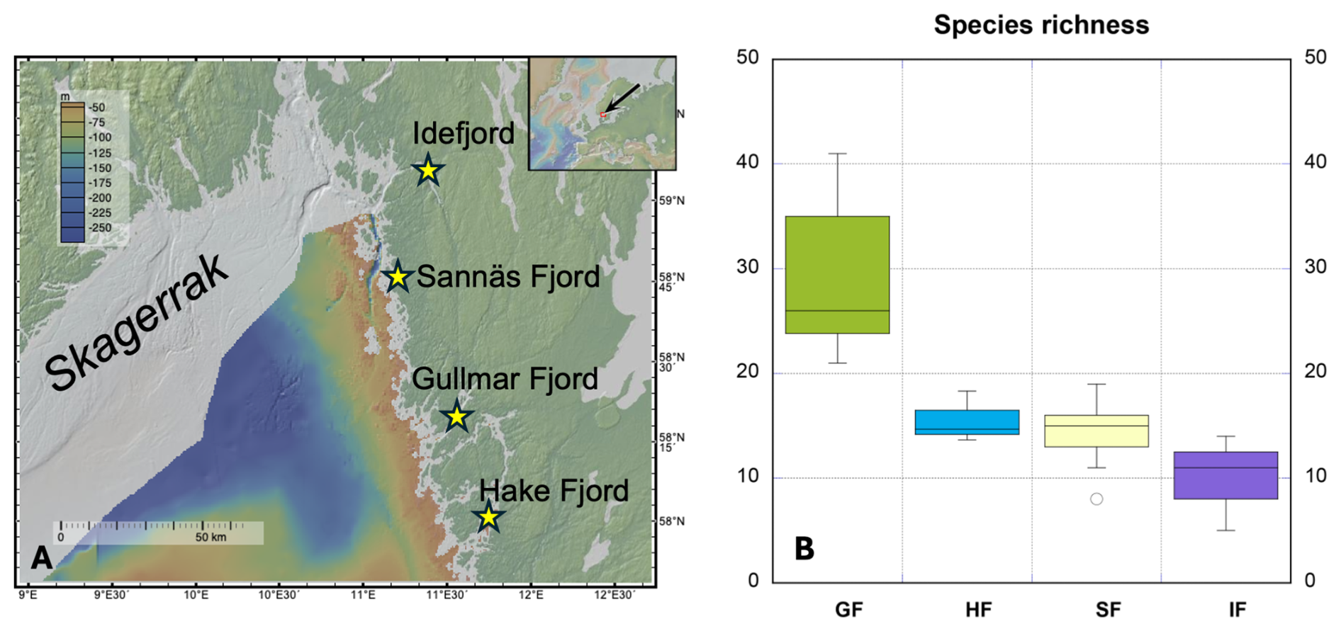
Figure 1 (a) Map over the Skagerrak fjords on the Swedish west coast, where the foraminiferal samples used in this study originate. The figure was created with GeoMapApp (http://www.geomapapp.org, last access: 10 October 2025)/CC BY. (b) Range of foraminifera species richness observed in the studied fjords showing clear diversity changes moving from the oceanic and deep-sea-like conditions (Gullmar Fjord) to progressively more estuarine conditions with increased riverine input (Idefjord). Abbreviations GF, HF, SF, and IF stand for Gullmar Fjord, Hakefjord, Sannäs Fjord, and Idefjord, respectively. Horizontal lines show median richness values.

The foraminiferal specimens were picked and mounted on micropaleontological slides (Fig. 2c). Prior to this, all sediment samples were washed over 63 and 1000 µm sieves and dried at 50 °C, and at least 300 individuals were picked from non-stained samples. No sample treatment was applied to concentrate foraminifera because of fjord sediments being composed of fine-grained organic-rich clay. The foraminiferal specimens were imaged using a Nikon SMZ-10 stereomicroscope equipped with a DeltaPix DP450 microscope camera (Fig. 2d). The camera provided a resolution of 1600×1200 pixels (1.92 MP), and images were captured at 30× magnification, resulting in an optical resolution of approximately 4.16 µm per pixel. To maintain consistency across images, the exposure time, lighting angle, light intensity, and magnification were kept as constant as possible throughout the imaging process. Light intensity was kept at the maximum of what the ring lamp could supply, and we opted for the ring lamp because the illumination with such a setup is more constant than with arm lights which can be bumped or moved during different imaging sessions. A total of 3095 sample images (each containing multiple individual specimens) were obtained over a 2-month period (Fig. 2e). The foraminifera in these images were oriented in various ways due to the use of both mounted (i.e., glued-on slides with fixed orientations) and non-mounted (i.e., not glued, with free movement allowed during manipulation) specimens, which proved beneficial for training the machine learning model. By capturing different views of each specimen, the model was better able to learn species-specific morphological features that might not be apparent from a single orientation.

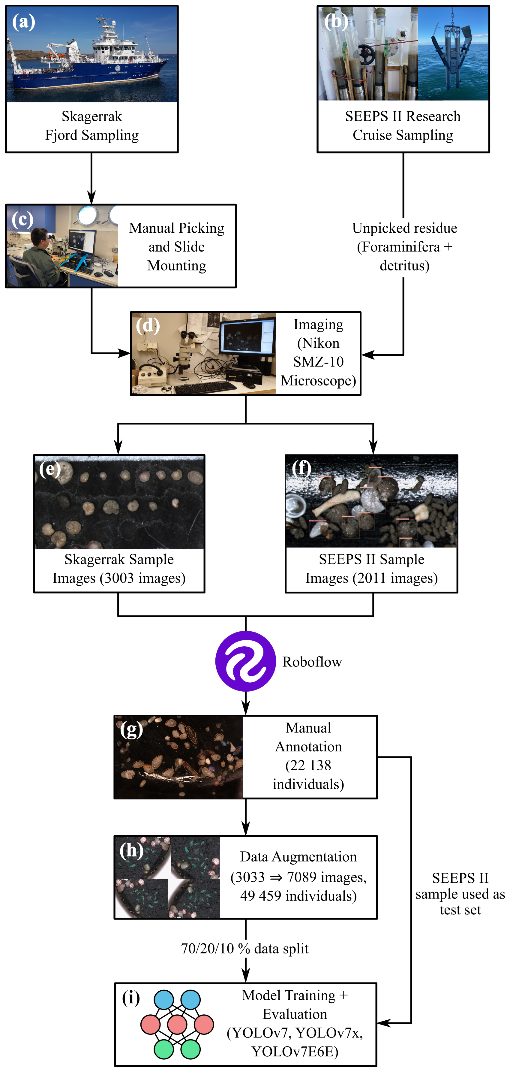
Figure 2 Analysis pipeline for training deep learning models using benthic foraminifera. The samples are sourced from two sampling initiatives: the Skagerrak fjord sampling (a) and the SEEPS II research cruise sampling (b). For the Skagerrak samples, benthic foraminifera were manually picked and mounted on slides (c). The SEEPS II samples were not manually picked and were instead imaged with foraminifera and detritus spread together in a picking tray. The samples were imaged using a Nikon SMZ-10 microscope (d), resulting in 3003 images from the Skagerrak sample (e) and 2011 images from the SEEPS II sample (f). Roboflow was then used to manually annotate 22 138 individuals from the combined samples (g). Data augmentation increased the number of images to 7089, resulting in a total of 49 459 individuals (h). This aggregated dataset was then split into training, validation, and test datasets ($\mathrm{70}/\mathrm{20}/\mathrm{10}$ % split) and used to train the YOLOv7, YOLOv7x, and YOLOv7E6E models (i). 

Additionally, during the SEEPS II research cruise conducted in April 2023, a second dataset of benthic foraminifera was prepared using surface sediment samples (> 63 mm fraction sediment residue) collected in the western Skagerrak and the Kattegat (Fig. 2b; 2011 images). This dataset was processed differently from the initial Skagerrak fjord dataset: the foraminifera were not picked; thus the samples containing both foraminifera and detrital material left after sieving were imaged from a micropaleontological tray (Fig. 2f). This provided an additional opportunity to evaluate the model's performance on real-world samples, as opposed to only on picked and cleaned specimens mounted on or stored in slides.

2.2 Image processing and labeling

The collected images were saved in TIFF format for high-quality preservation, as this format does not compromise image quality due to compression artifacts. These images were then processed using Roboflow, a web-based application programming interface (API) designed for machine learning tasks. Roboflow allows users to easily label images and create datasets suitable for training machine learning models (Fig. 3). One of the most valuable features of Roboflow is its content-aware selection tool, which automatically detects the boundaries of objects, significantly reducing the time required for manual labeling. A total of 22 138 individual foraminifera were manually labeled across the dataset by the first author over a 2-month period (Fig. 2g). On average the first author spent 1 h labeling per working day, equaling ∼ 80 h total. The labeling process involved manually drawing polygons around each foraminifera specimen in the images and assigning a species label to each specimen. This labeled dataset was then exported for use in model training.

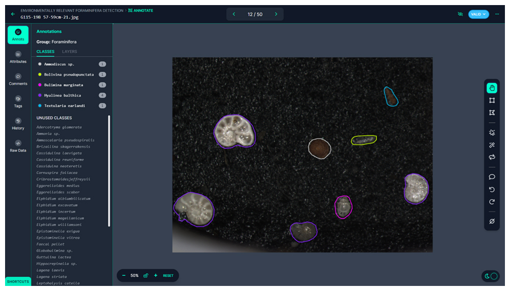
Figure 3 Roboflow interface for classifying individual foraminifera in an image. On the left side of the window, there is a color-coded list of labeled foraminifera in an image on the right. On the rightmost side, there is a tool selection panel, from which a user can label foraminifera either by using an automatic feature extraction tool or by manually drawing a polygon around the foraminifera. In this study, the specimens were labeled using manually drawn polygons.

2.3 Dataset creation

Once the images were labeled, the dataset was split into three subsets ($\mathrm{70}/\mathrm{20}/\mathrm{10}$ %) for the training, validation, and testing sets, respectively. In total, 3003 images were used to create the dataset, containing 22 138 labeled individuals. However, not all species identified in the original sediment samples were included in the training dataset. Out of 59 identified species, 29 species were chosen for training (Fig. 4). The remaining 30 species were excluded due to having too few labeled individuals (fewer than 72 individuals), which could have reduced the accuracy of the model during training. The cutoff point for species inclusion was set at 72 labeled individuals based on initial model testing. Model performance for those less abundant species with an individual count lower than 72 resulted in precision less than 0.5; therefore only species with precision higher than 0.5 were included.

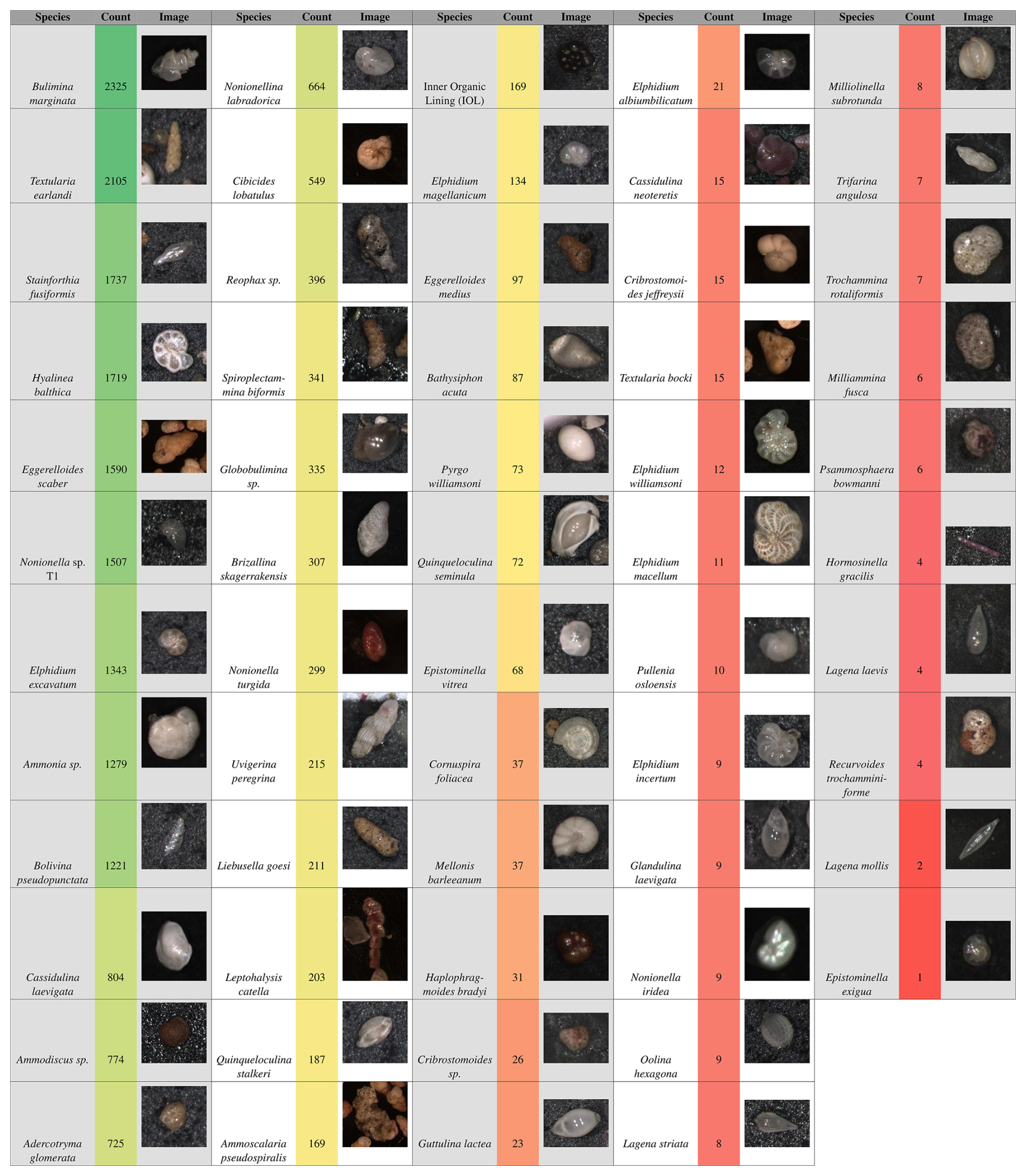
Figure 4 List of all benthic foraminifer species imaged in this study, with total counts and representative images. Of the 50 total species imaged, 29 were selected for training the model (those with ≥ 72 images; Quinqueloculina seminula and above).

To increase the effective size of the dataset, data augmentation techniques were applied (Fig. 2h). Data augmentation involves making systematic changes to the images, such as adjusting brightness, contrast, and vibrance, as well as horizontally and vertically flipping the images. The augmentations used in this work included flipping the images horizontally and vertically and rotating them 90° clockwise, counter-clockwise and upside down. Hue, vibrance, brightness, and exposure were adjusted randomly between −25 % and +25 %. Artificial noise was added up to 5 % of total pixels. These augmentations create new versions of the original images that are slightly different from each other, allowing the model to learn to recognize species under varying conditions. After augmentation, the dataset contained 7089 images and 49 459 labeled foraminifera. As the augmentation process was done after annotation, it did not require additional manual annotation, as the annotations from the original images were retained.

2.4 Object detection with You Only Look Once (YOLO)

Unlike object detection methods which rely on sliding windows or region proposals, such as Mask-RCNN (He et al., 2017), YOLO models divide the input image into a grid and predict bounding boxes and class probabilities for each grid cell simultaneously. This allows YOLO to detect objects in a single forward pass through the network, significantly reducing computation time (Wang et al., 2023). YOLOv7, the version used in this study, builds on previous iterations by improving detection accuracy through reparametrized convolutions and model scaling (Wang et al., 2023). These innovations enable YOLOv7 to perform well on complex datasets while maintaining fast processing times. The model is particularly efficient in detecting small objects, which is a critical feature for identifying foraminifera in images taken from micropaleontological slides, where the minute organisms are non-mounted and can be closely packed together.

In this study, YOLOv7 was chosen for its balance between speed and accuracy based on its performance on the Common Objects in Context (COCO) dataset, a standard dataset for computer vision model evaluation and benchmarking (Lin et al., 2014). To find an optimal model it is important to look at their average precision (AP), which measures accuracy of the model, and to look at batch 1 frame per second (FPS) and batch 32 average time (Table 1). Batch 1 FPS measures frames per second when processing one image at a time. Higher FPS means faster processing, indicating that the model can process images more quickly. Such performance is valuable for real-time applications. Batch 32 average time measures the average time needed to process a batch of 32 images in milliseconds. Lower times are better as they indicate faster processing, valuable for processing images and videos. The model's ability to detect multiple objects in a single image makes it ideal for processing large datasets of benthic foraminifera, where multiple individuals may be present in each frame. The use of YOLOv7 also allows real-time detection applications, which could potentially be extended to mobile or desktop-based tools for species identification in the future.

Table 1 A comparison of YOLOv7 models' performance on the COCO dataset (Lin et al., 2014) prior to the training with foraminifera images.

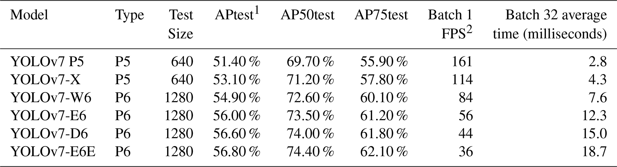
¹ AP: Average precision. ² FPS: Frames per second, a measure of the frequency (rate) at which consecutive images are captured or displayed.

2.5 Transfer learning for small datasets

One of the challenges in applying deep learning models to ecological datasets is the relatively small size of the datasets compared to those typically used in fields like computer vision. In this study, the dataset consisted of 3003 images with 22 138 labeled individuals, which is relatively small compared to large-scale datasets like ImageNet (Deng et al., 2009) or the COCO database (Lin et al., 2014), which contain millions of labeled images. Training deep learning models from scratch on such small datasets can lead to overfitting, where the model memorizes the training data but performs poorly on new, unseen data (i.e., poor generalizability). To address this issue, transfer learning was used in this study. Transfer learning involves using a model that has already been trained on a large dataset for a different task and fine-tuning it for a new task with a smaller dataset (He et al., 2015). In the case of YOLOv7, the model was pre-trained on the COCO database (Table 1), which contains a diverse set of objects from everyday scenes. By starting with a model that already “knows” how to detect general objects, we can fine-tune it to recognize specific objects like foraminifera with far fewer training images. This approach allows the model to leverage the knowledge it gained from the large dataset and apply it to the new task, thereby improving its performance even with a relatively small training set. In this study, transfer learning was used to initialize the weights of the YOLOv7 model before training it on the benthic foraminifera dataset. This enabled the model to achieve high accuracy despite the limited number of labeled data available.

2.6 Model training

For this study, three different models from the YOLOv7 family were trained: YOLOv7, YOLOv7x, and YOLOv7E6E (Fig. 2i). These models differ in their architecture, the number of layers, and the size of the input images they can process. YOLOv7 and YOLOv7x use 640 × 640 pixel images as input, while YOLOv7E6E uses 1280 × 1280 pixel images, which allows it to detect smaller objects in greater detail. All models were trained on a workstation equipped with an Intel i7 9700K processor (8 cores, 8 threads at 3.60 GHz), 32 GB of RAM, and a Nvidia RTX A4000 graphics card running Kubuntu 22.04. The models were trained using the PyTorch deep learning framework (version 2.0.0) with CUDA version 11.7 for GPU acceleration.

The training process consisted of 350 epochs for each model (one epoch = one complete pass of the entire training dataset through the CNN). The smallest model (YOLOv7) took approximately 18 h to train, the medium-sized model (YOLOv7x) took 25 h, and the largest model (YOLOv7E6E) required 120 h due to its increased complexity and higher input resolution. During training, the model weights were initialized using pre-trained weights from the COCO dataset and fine-tuned through subsequent training sessions.

2.7 Object detection metrics

In object detection tasks, model performance is typically evaluated using several key metrics, including precision (P), recall (R), and Intersection over Union (IoU). Precision measures the proportion of correctly identified objects (true positives) out of all positively identified objects, while recall measures the proportion of true positives out of all actual objects in the image, i.e.

$$\begin{array}{}\text{(1)}& {\displaystyle }\text{precision}={\displaystyle \frac{\mathrm{TP}}{\mathrm{TP}+\mathrm{FP}}}\text{(2)}& {\displaystyle }\text{recall}={\displaystyle \frac{\mathrm{TP}}{\mathrm{TP}+\mathrm{FN}}},\end{array}$$

where TP = true positives, FP = false positives, and FN = false negatives. IoU is used to quantify the overlap between the predicted bounding box and the ground truth bounding box, with higher IoU values indicating better accuracy at a given threshold value (Fig. S1 in the Supplement).

These metrics can be combined to compute more comprehensive performance indicators such as average precision (AP) and mean average precision (mAP). AP is the area under the precision–recall (PR) curve, which plots precision on the y axis and recall on the x axis for different confidence thresholds. In turn, mAP is calculated as the average of the AP values over all classes (i.e., species) and is commonly used to evaluate the overall performance of object detection models (Padilla et al., 2021).

For this study, the performance of the trained YOLOv7 models was evaluated using mAP at two different IoU thresholds: 0.5 (mAP@0.5) and 0.5 to 0.95 in steps of 0.05 (mAP@0.5:0.95). The threshold of 0.5 is commonly used as a standard measure of detection accuracy, while the 0.5:0.95 range provides a more stringent evaluation by considering a range of IoU values.

The F₁ score was also used to evaluate model performance. The F₁ score combines precision and recall into a single metric and is particularly useful for evaluating models with unbalanced datasets. It is the harmonic mean of precision and recall and is defined as

$$\begin{array}{}\text{(3)}& F_{\mathrm{1}}={\displaystyle \frac{\mathrm{2}\times \mathrm{TP}}{\mathrm{2}\times \mathrm{TP}+\mathrm{FP}+\mathrm{FN}}}.\end{array}$$

In this study, the confidence threshold was adjusted to maximize the F₁ score, which maximizes precision and recall simultaneously.

3 Results

3.1 Model training and performance overview

Over the course of the study, 58 training experiments were conducted using different configurations of the YOLOv7 architecture (Table S1 in the Supplement). Out of these, 23 models were successfully trained, while the remaining 35 failed due to memory limitations. We used the default YOLOv7 experiment suffix, “exp”, for the name of each experiment. Models exp 10 and exp 50 used a 16-image batch size, while exp 56 and 58 used an 8-image batch size. The E6E models exp 51, 52, and 53 used only a 2-image batch size. These batch size differences result from the amount of space taken up in GPU memory by the different model types, with the E6E model being the largest. The best-performing models are summarized in Table 2. Out of these, the best-performing model was exp 50, which achieved a precision of 0.877, a recall of 0.882, and a mean average precision (mAP) of 90.3 % at an IoU threshold of 0.5 and 69.9 % at a threshold range of 0.5 to 0.95. The model was based on the YOLOv7x architecture using 640 × 640 pixel images as input.

Table 2 Performance comparison of trained models.

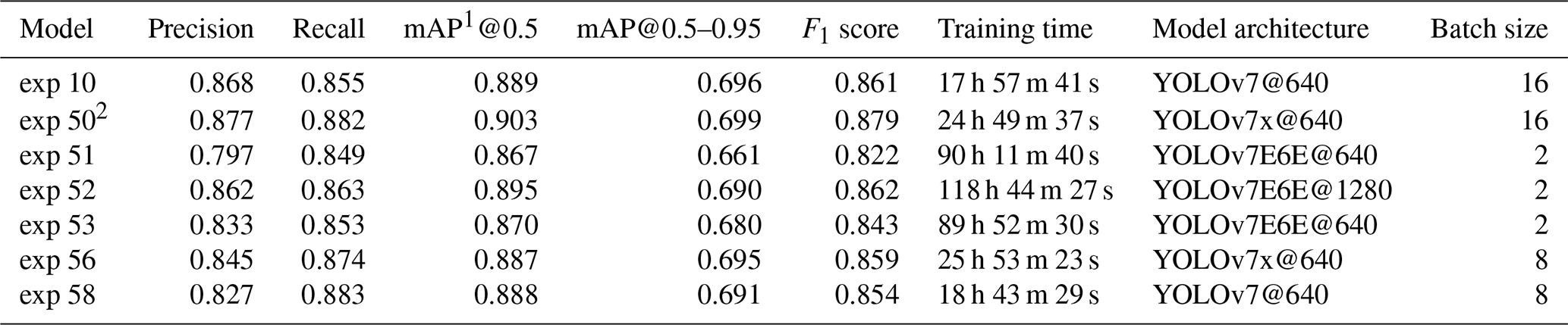
¹ mAP: mean average precision. ² Best-performing model

3.2 Training curves

The performance of the models was monitored throughout the training process using loss curves, which provide insight into model performance across training epochs. Figure 5 shows examples for the training curves for exp 50, which include three types of loss: box loss, objectness loss, and classification loss.

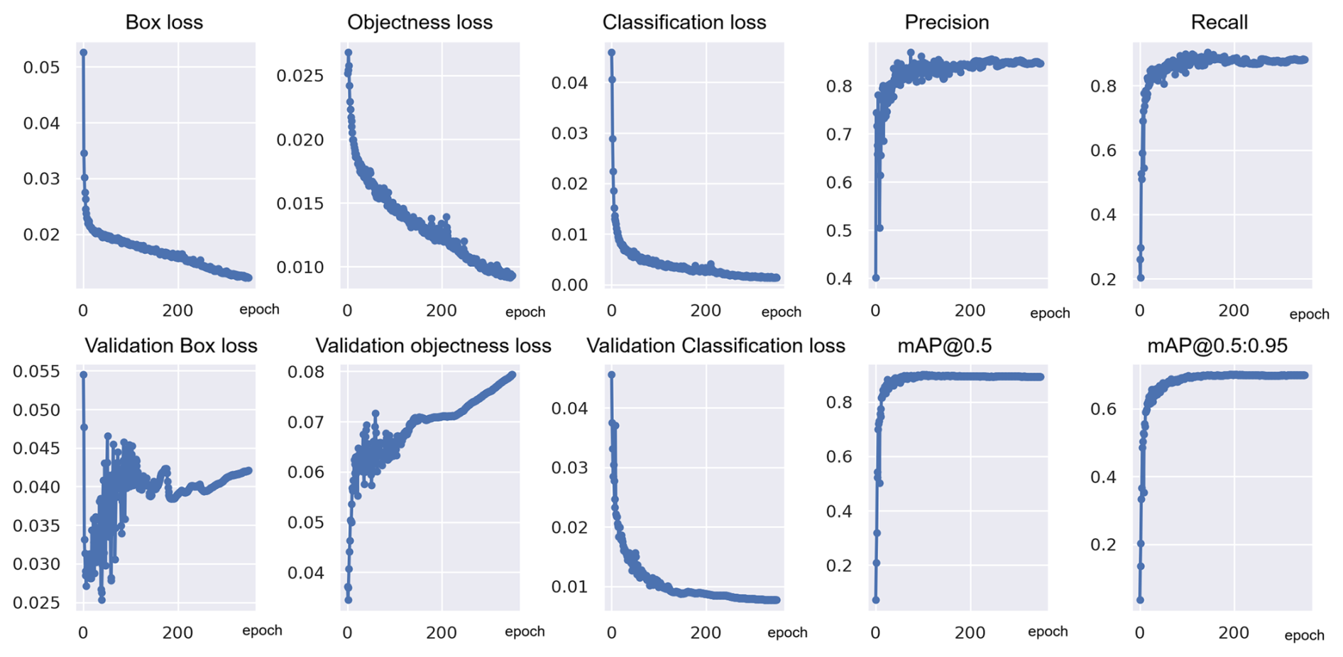
Figure 5 Training and validation curves for the best-performing model, exp 50, showing box loss, objectness loss, classification loss, precision, recall, and mean average precision (mAP) (corresponding y axes) across training epochs (x axes).

Following the definitions of Alexe et al. (2012):

• Box loss measures how accurately the model can predict the location and size of bounding boxes around detected objects. The lower the box loss, the higher the model accuracy generally, but the model must also correctly classify objects and avoid false positives and negatives.

• Objectness loss represents the probability that an object exists within a given region of interest. If objectness is high, it indicates that the model exists within a given region, while a low objectness score indicates that the region is background or that it does not contain any object of interest.

• Classification loss measures how well the model can classify the detected objects into the correct species category. The lower the classification loss, the higher the model accuracy generally, but the model must also optimize objectness and box loss to achieve high accuracy in all respective categories.

During training, the loss values decreased steadily over time, indicating that the model was learning to better detect and classify foraminifera species (Fig. 5). For classification, the validation loss closely followed the training loss, suggesting that the model did not suffer from significant overfitting.

3.3 Confusion matrix

The confusion matrix (Fig. 6) provides a detailed view of the model's classification performance by showing the number of correct and incorrect predictions for each species on the test set of images. Figure 6 displays the confusion matrix for the best-performing model, exp 50.

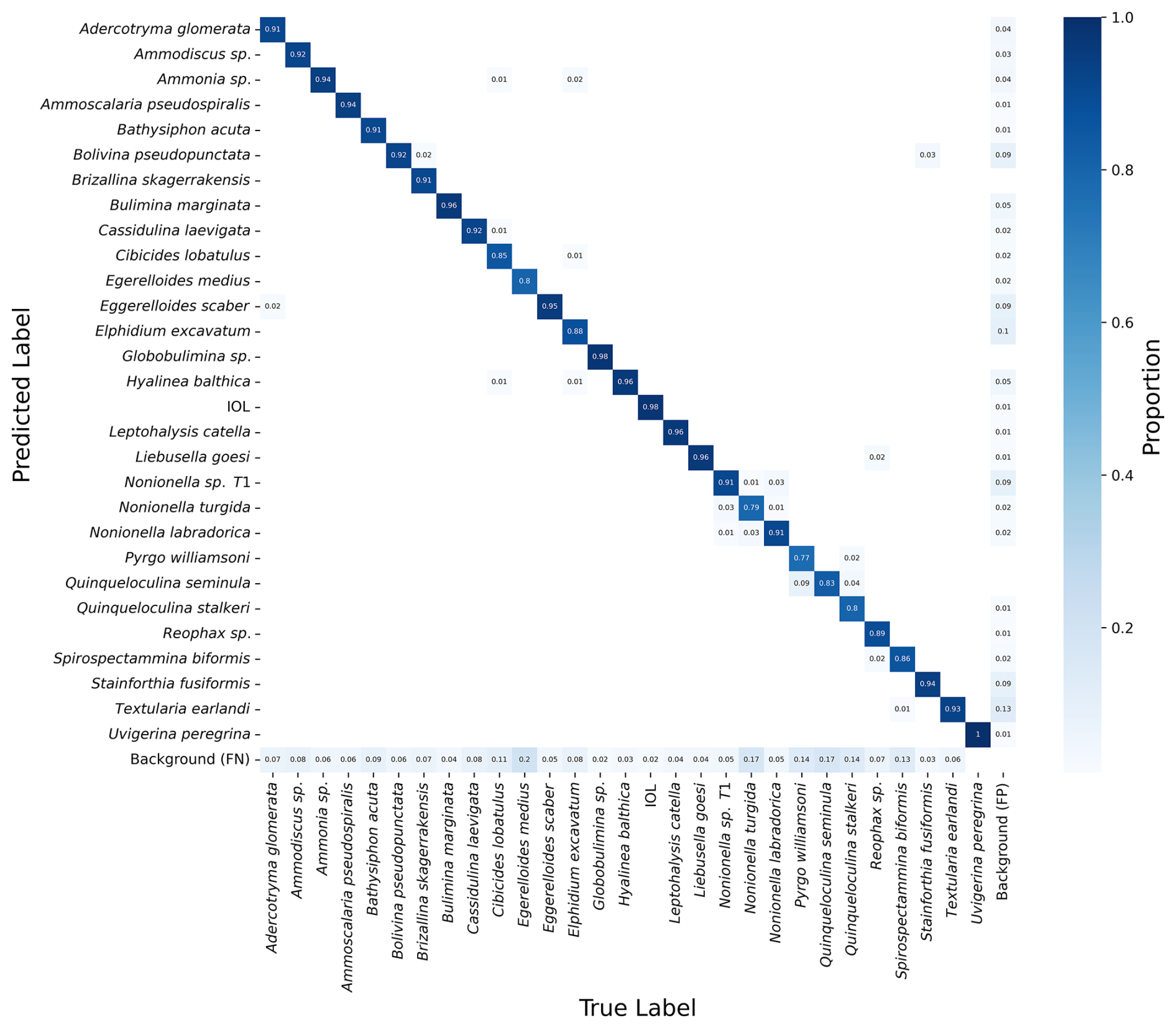
Figure 6 Confusion matrix of the best-performing model, exp 50. On the left-hand side are the predicted labels made by the model, and on the bottom of the matrix are the ground truth labels. The shade of blue indicates the proportion of images in the test set that the model correctly identified as the given species (only values > 0 are shown). The model has false negatives of background in all species, while mistaking only a small percentage of one foraminifera species with other foraminifera species. IOL: inner organic lining; FN: false negative; FP: false positive.

The confusion matrix reveals that the model performed well across most species, with most predictions falling along the diagonal (correct classifications). However, there were some instances where the model confused species with similar morphology. For example, species in the genus Nonionella and Eggerelloides were occasionally misclassified, reflecting the challenge of distinguishing between species within the same genus and with subtle morphological differences.

The matrix also shows that the model had a small number of false positives and false negatives for the background (1 %–13 %), indicating that it sometimes incorrectly identified sediment particles or other debris as foraminifera (Fig. 6).

3.4 Object detection metrics

Figure S2 shows the precision and recall results for the best-performing model, exp50. At a confidence threshold of 0.540, the model achieved its highest F₁ score (Fig. S2a), indicating a balanced trade-off between precision and recall. This threshold was used in subsequent evaluations of the model's performance. The precision–recall (PR) curve (Fig. S2b) provides a visualization of the model's precision and recall across different confidence thresholds. A high area under the PR curve indicates strong performance, with both high precision (low false positive rate) and high recall (low false negative rate).

The precision and recall curves (Fig. S2c, d) provide additional insights into the model's behavior during training. Typically, as the confidence threshold increases, precision increases while recall decreases. The precision curve shows that precision increases as the confidence threshold increases, indicating fewer false positives at higher confidence levels.

The recall curve shows that recall decreases as the confidence threshold increases, indicating fewer false negatives at lower confidence levels. The model provided output images (Fig. 7), where the input image of benthic foraminifera is processed by the model, resulting in an output image with bounding boxes and species labels. The confidence level of the model predictions is displayed next to each species name (Fig. 7).

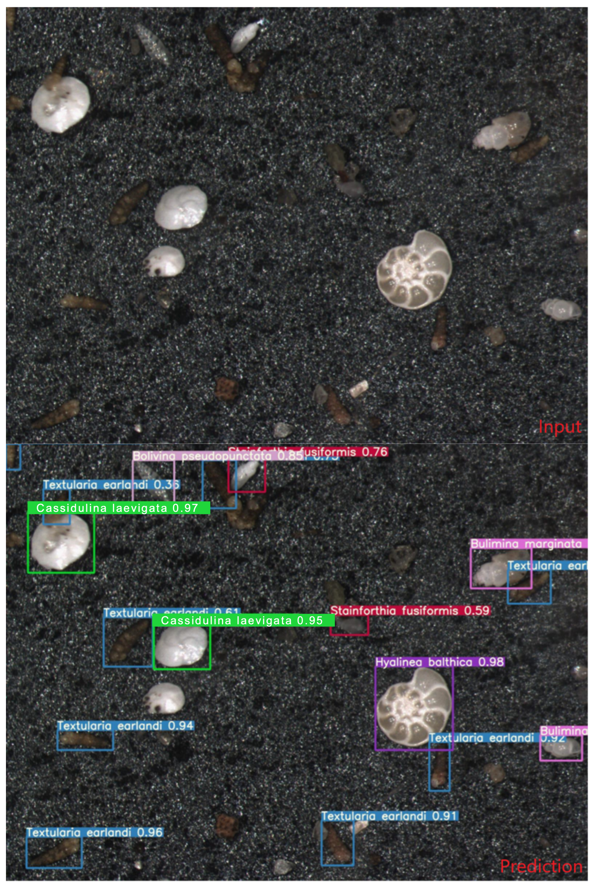
Figure 7 Input image of foraminifera (top figure) is processed by a model and creates a new image (bottom figure) with bounding boxes and species name. The number next to the species is the confidence level of the model between 0–1.

4 Discussion

4.1 Performance of the YOLOv7 and comparison with existing models

While YOLO family models have been used on other microfossils including ichthyoliths (Mimura et al., 2024), fish scales (Hanson et al., 2024), and pollen (Kubera et al., 2022; Endo et al., 2024; Jofre et al., 2025), to the best of our knowledge this study is one of the first to apply the YOLO architecture to the identification of foraminifera as of time of writing and is one of the very few models used on benthic foraminifera specifically to date. The results from this study demonstrate that deep learning, specifically the YOLOv7 family of models, can be effectively applied to the task of benthic foraminifera identification from the diverse species communities such as in the Skagerrak fjords. Among the models tested, YOLOv7x (exp 50) performed the best, achieving a mean average precision (mAP) of 90.3 % at an IoU threshold of 0.5 % and 69.9 % at the stricter 0.5 to 0.95 range. These results are competitive with, and in some cases exceed, the performance of other machine learning models that have been used for foraminifera identification (Table 3). For instance, Hsiang et al. (2019) employed a VGG16 CNN to classify 35 planktonic foraminiferal species, achieving a precision of 87.4 %. Their study led to the creation of the Endless Forams dataset, which included over 34 000 individual foraminifera. This dataset was then used by Karaderi et al. (2022) to train a deep metric learning model which achieved an accuracy of 92 % at an F₁ score of 0.84. Although these studies focused on planktonic species, the performance of the VGG16 and deep metric learning models is comparable to the YOLOv7x model used in this work, which both achieved a precision of 87.7 % and an mAP@0.5 of 90.3 %, respectively.

Table 3 Overview of deep learning classification models applied to foraminifera discussed.

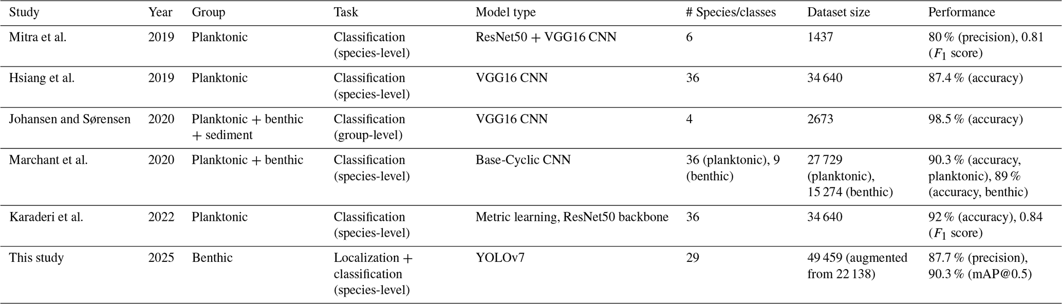
Similarly, Marchant et al. (2020) used a customized ResNet50 model on the Endless Forams dataset, achieving a precision of 90.3 %. This model was also trained on both planktonic and benthic foraminifera, with a slightly lower precision of 89 % for the benthic species. While the precision achieved by Marchant and colleagues is higher than the YOLOv7x model on some species, the key advantage of YOLO lies in its ability to perform object detection in addition to classification. This makes YOLO suitable for scenarios where foraminifera need to be identified within unpicked sediment samples that contain non-foraminifera objects, which would typically require manual sorting before classification to reduce task complexity. In another study, Mitra et al. (2019) combined ResNet50 and VGG16 models to classify planktonic foraminifera, achieving a precision of 80 %. The lower precision in their study can be attributed to the smaller dataset of 1437 individuals, highlighting the importance of dataset size for model performance. In contrast, the dataset used for the YOLOv7x model in this study was augmented to include over 7000 images, leading to improved performance. Johansen and Sørensen (2020) implemented a VGG16 model for the classification of both sediment particles and benthic foraminifera, achieving a 98.5 % precision for this simpler task of detecting and differentiating between broad categories. However, the focus of their model was not species-level classification, and its application is limited to basic detection tasks, whereas the YOLOv7x model presented in this study demonstrates significant capabilities for species-level identification.

One key factor contributing to the success of the YOLOv7x model is its ability to balance detection accuracy with speed. YOLO models, in general, are designed to process images in a single forward pass, making them exceptionally fast compared to other object detection algorithms. For example, Wang et al. (2023) show that the base YOLOv7 model is more than 6 times faster than the fastest non-YOLO model tested (Deformable DETR), with an FPS of 118 vs. 19 on a V100 GPU. This makes them ideal for real-time applications and for processing large datasets efficiently. The inclusion of YOLOv7E6E, which accepts larger input images (1280 × 1280 pixels), showed that increasing image resolution improved detection in some cases but at a significant computational cost. As a result, the YOLOv7x model has shown the most promise for use in real time applications, since its high inference speed allows it to be used directly during foraminifera picking (for instance, allowing non-experts to pick specimens when training students or future applications using robotics) owing to its fast frame-per-second performance (≈ 65 FPS). However, the integrated nature of the YOLO workflow (i.e., the identification and segmentation steps are combined into a single, one-step model) does present some disadvantages in comparison to two-step workflows (i.e., a segmentation model is trained first to localize objects, followed by a separate classification model to perform identification) (not to be confused with one- vs. multi-stage segmentation models, e.g., YOLO vs. Mask RCNN). The latter has been shown to perform advantageously in problems varying from skin lesion identification (Shakya et al., 2025) to the identification of diatoms in sediment traps (Godbillot et al., 2025) and allows a separate evaluation of problems in segmentation and classification. The trade-off between speed/computational cost (in which one-step models are advantaged) and accuracy (in which two-step models are advantaged) must be balanced when determining the most suitable model type for a particular task. For instance, it would likely be preferable to use YOLO-type models for rapid, in situ, real-time biomonitoring applications. On the other hand, tasks that involve samples that must be substantially pre-processed (e.g., coretop sediment samples) – resulting in the analysis bottleneck being centered on sample preparation and imaging – might be better served by higher-accuracy two-step models. We note that our results show that one of the classical drawbacks of YOLO models – poor performance with small objects (Tariq and Javed, 2025) – does not appear to significantly impact accuracy in this case.

4.2 Species-level performance

While the overall performance of the YOLOv7x model was strong, there were notable variations in its species-level performance. For common species such as Nonionellina labradorica and Bulimina marginata, precision and recall values exceeded 90 %, indicating the model's robustness in detecting and classifying species with abundant training data. However, for less abundant species like Eggerelloides medius, performance was notably lower, with a precision of 55.3 %. This discrepancy can largely be attributed to the limited number of training examples for these less abundant species, which is a common challenge in supervised learning models (Table S2).

In the case of Eggerelloides medius, the confusion with morphologically similar species, such as Eggerelloides scaber, highlights one of the primary limitations of the current model: its limited ability to differentiate between closely related species. This issue is exacerbated by the presence of subtle morphological differences that may not be sufficiently captured in lower-resolution images or that require more nuanced feature extraction techniques. Future work could address this limitation by incorporating higher-resolution images and additional morphometric data or by using hybrid models that integrate both image and textural data. Our data additionally show that the model struggled with certain species, particularly agglutinated foraminifera like Eggerelloides medius and Textularia earlandi. These species are characterized by their relatively simple yet irregular shell structures, which may have been more difficult for the model to distinguish against the dark background of microslides.

Generally, it appears that common denominators of poor performance of the model are:

• a.

  agglutinated species, which the model has difficulty distinguishing against the black background;

• b.

  large and voluminous (e.g., globular to spherically shaped) species, which require multiple focal points to distinguish details needed for accurate identification; and

• c.

  species with a low number of individuals in the training set (fewer than 100 individuals).

Another challenge observed in the confusion matrix of this study was the tendency for background elements to be misclassified as foraminifera in some instances, contributing to a false positive rate of 1 % to 13 % across different species. While this issue was relatively minor in comparison to the overall performance, it underscores the importance of careful image pre-processing and the potential value of incorporating background filtering algorithms or the use of different background colors to further enhance the model's accuracy.

4.3 Applications and implications

One of the key advantages of the YOLOv7 architecture is its ability to process images in real time, which opens new possibilities for automated species identification in the field. For example, researchers could deploy YOLO-based models on applications for mobile devices or desktop computers to identify foraminifera in real time during fieldwork or laboratory analysis. This would significantly reduce the time and expertise required for species identification, making it accessible to a broader range of users.

Additionally, the ability to identify foraminifera directly from unpicked sediment samples represents a major advancement in foraminiferal studies. Current methods for analyzing foraminifera require time-consuming manual sorting and picking of individual specimens, which limits the scalability of environmental monitoring programs. By applying deep learning models to sieved sediment samples that have yet to be picked for foraminifera, researchers can streamline the analysis process and obtain results more quickly, allowing more frequent and widespread monitoring of marine ecosystems.

4.4 Limitations and future directions

While this study demonstrates the effectiveness of deep learning for foraminifera identification, there are several limitations that should be addressed in future work. One limitation is the relatively small size of the dataset, particularly for certain species. As noted earlier, species with fewer than 100 labeled individuals tended to perform worse in the model, likely due to the lack of sufficient training data. Future studies should aim to increase the size and diversity of the dataset, either by collecting more images through taking multiple images of the same individual from multiple angles or by augmenting the existing data through additional augmentation techniques. The model results presented here also point the way for future targeted sampling initiatives, as species with lower identification accuracies are clearly demarcated.

Another limitation is the use of a single imaging setup, which could introduce bias into the model. All images in this study were captured under the same lighting and magnification conditions, which may limit the model's ability to generalize to images taken under different conditions. In future studies, it would be beneficial to test the model on images collected using different microscopes, cameras, or lighting setups to evaluate the model's robustness to varying conditions. Additionally, the use of different background colors for microscopic slides could prove beneficial for distinguishing boundaries between foraminifera specimens and the background. One potential background color could be chroma key green, which has shown considerable success in the movie industry for decades in the visual effects field. Further, the use of z-stacking, which would provide higher-resolution images by incorporating multiple focal planes, would allow a deep learning model to learn to recognize species-specific features that are not visible or resolved in a single 2D image. This would be particularly useful for large individuals that exceed a given camera's depth of focus. While z-stacking is a standard component of many microfossil imaging pipelines (e.g., Elder et al., 2018; Hsiang et al., 2019; Marchant et al., 2020; Adebayo et al., 2023), incorporating z-stacking necessitates a corresponding increase in imaging time and file sizes (proportional to the number of slices taken). Furthermore, additional hardware and software are required, particularly for large imaging initiatives (e.g., automated microscope stages), which may be a limiting factor depending on funding and accessibility. The fact that we achieve high accuracies in this study without using z-stacking is notable, and it suggests that useful training data can be collected for species identification even when the imaging setup is not optimized for image resolution and quality.

While this study represents an important step forward in the use of automated segmentation models for rapid identification of benthic foraminifera, there remain many avenues for future work as we endeavor to develop such models for application in biomonitoring. These directions for future work include improving the model architecture, improving the training dataset (including incorporating metadata to enhance model accuracy), and expanding model deployment. The YOLO model used in this study, YOLOv7, is only one in a family of models that enjoys good support from developers and continued research interest; since the experimental part of this study was completed, as of the time of writing, there have been four new updates to the architecture, with the current version being YOLOv11 (Jocher and Qiu, 2024). This new model shows further improvements in object detection and inference time compared to its predecessors (Khanam and Hussain, 2024). In addition to using newer model architectures, future work could explore the use of ensemble learning techniques, where multiple models are combined to improve overall classification accuracy. By integrating the strengths of different architectures – such as YOLO models for object detection and ResNet or VGG models for fine-grained classification – it may be possible to achieve even higher precision and recall, particularly for challenging cases involving similar species.

While using alternate model architectures would likely improve accuracies, in certain cases one might be limited in one's model choice by hardware availability; for example, in this study, many of our experiment setups were not feasible due to the lack of sufficient GPU memory to implement larger models (e.g., YOLOv7E6E; Table S1). As such, other ways of improving model performance should also be considered. One of the most important of these which is often overlooked is the quality of the actual training data. In this case we are referring not to the image quality (as in the discussion on z-stacking above) but to the quality of the annotations and labeling. To our knowledge, a systematic review of annotation practices for building species identification training sets does not yet exist (and is outside the scope of this study). However, it is our general observation that most studies training models for species identification, including this one, use training datasets that have been labeled/annotated by a single worker or equivalent (i.e., multiple workers that label non-overlapping image sets). This is often done to save time on annotation, which is a time-consuming manual process. However, having only a single labeler means that annotation mistakes are difficult to catch and are likely to be propagated through to training, leading to systematic biases. Hsiang et al. (2019) prioritized training set quality for the Endless Forams dataset by having all images labeled by four independent experts and only retaining images for which there was ≥ 75 % agreement on the species identity for the final training dataset. While such annotation procedures would be preferable, there is a significant trade-off in time spent annotating unless a large team can be assembled to label (as in the case of the Endless Forams study). This type of annotation strategy also requires agreement on a community taxonomy to which all labelers agree to adhere. While the current study serves as a promising proof of concept, initiatives moving forward must carefully consider their labeling procedures in order to minimize systematic biases in their training sets.

Another data-based approach to improving model performance is the incorporation of metadata together with image data in fused networks. Previous work has shown that data fusion of this kind, where camera trap images are combined with metadata such as location, improves model accuracy (Tøn et al., 2024). The integration of molecular data, such as species barcoding and metabarcoding (eDNA) data, could also enhance the accuracy of species identification models. Recent (non-deep-learning) studies have shown that combining morphological and genetic data can significantly improve the resolution of species identification in foraminifera, particularly for cryptic or closely related species (e.g., Darling et al., 2016; Bird et al., 2020; Richirt et al., 2021). Future studies should explore the potential of combining deep learning models with molecular techniques to develop more comprehensive tools for environmental monitoring. Additionally, since the detection of dead vs. living material is important for bioindicator applications, an important avenue for future work is the incorporation of stained (e.g., rose bengal) and/or labeled (e.g., CellTracker Green) individuals in the training dataset.

5 Conclusions

This study demonstrates the effectiveness of using deep learning models, specifically YOLOv7x, for the automated identification and classification of benthic foraminifera from the Skagerrak Fjords. The YOLOv7x model achieved high performance metrics, with a precision of 87.7 %, a recall of 88.2 %, and a mean average precision (mAP@0.5) of 90.3 %. These results suggest that deep learning models can significantly reduce the time and effort required for foraminiferal identification, offering a faster and more scalable solution compared to manual methods.

The two most important contributions of this study are as follows:

1. Automation of species-level classification. This study is one of the first to apply YOLOv7 to benthic foraminiferal classification, successfully automating the identification process while maintaining accuracy comparable to expert manual identification. By leveraging deep learning, it is possible to process thousands of images in minutes, a task that would typically take days or weeks with manual analysis.

2. Comparison to existing models. When compared to other models, such as VGG16 and ResNet50, which have been used in earlier studies, the YOLOv7x model presented here achieves competitive precision while offering the additional benefit of object detection, a critical feature for handling complex, unpicked samples.

In conclusion, the application of deep learning, specifically the YOLOv7x model, represents a significant advancement in the field of foraminiferal research. This study illustrates the potential of deep learning to automate and accelerate the process of species identification, making it more accessible for large-scale environmental monitoring. While challenges remain, particularly regarding underrepresented species, the findings presented here offer a strong foundation for future research and model improvement.

Lastly, this study does not aim to eliminate human expertise from the taxonomic identification process. Instead, an ML-based approach could be used as a labor-saving device to go through the bulk of the dataset, and later a person could validate and, if needed, correct the identifications. By reducing the time needed to identify foraminifera, one could focus more on the analysis of ecological interactions between the species.