the Creative Commons Attribution 4.0 License.
the Creative Commons Attribution 4.0 License.
 | 15 Oct 2020
Automated analysis of foraminifera fossil records by image classification using a convolutional neural network
Martin Tetard
Adnya Pratiwi
Michael Adebayo
Thibault de Garidel-Thoron
Manual identification of foraminiferal morphospecies or morphotypes under stereo microscopes is time consuming for micropalaeontologists and not possible for nonspecialists. Therefore, a long-term goal has been to automate this process to improve its efficiency and repeatability. Recent advances in computation hardware have seen deep convolutional neural networks emerge as the state-of-the-art technique for image-based automated classification. Here, we describe a method for classifying large foraminifera image sets using convolutional neural networks. Construction of the classifier is demonstrated on the publicly available Endless Forams image set with a best accuracy of approximately 90 %. A complete automatic analysis is performed for benthic species dated to the last deglacial period for a sediment core from the north-eastern Pacific and for planktonic species dated from the present until 180 000 years ago in a core from the western Pacific warm pool. The relative abundances from automatic counting based on more than 500 000 images compare favourably with manual counting, showing the same signal dynamics. Our workflow opens the way to automated palaeoceanographic reconstruction based on computer image analysis and is freely available for use.
- Article
(7279 KB) - Full-text XML
- BibTeX
- EndNote


Foraminifera are cosmopolitan unicellular marine protists that secrete unique carbonate shells, mostly on the submillimetre scale, that accumulate on the ocean floor, forming kilometres of carbonate sediment oozes. This long geological record gives foraminifera a variety of geological uses, such as in palaeoceanographic studies. For example, sediment cores provide a record of foraminiferal species composition and abundance over time, and the presence of a species can be used to date marine sediments for biostratigraphy. The relative and absolute abundances of different species, along with their morphometric characteristics and geochemical composition, have been used for decades as proxies for reconstructing past climate conditions, such as the temperature, oxygen concentration and salinity of oceans (e.g. Kucera, 2007). In pre-Quaternary studies, the ability of foraminifera records to track environmental changes make them widely used in biofacies definitions, a powerful tool to understand the structure of sedimentary deposits and their evolution through time. Their wide range of evolutionary rates are also an asset used for biostratigraphical studies, and planktonic foraminifera count among the main markers of the geological timescale (Gradstein et al., 2012). Lastly, the extremely wide range of environments colonized by foraminifera, from the deep sea to the shallow shelves and the oligotrophic surface ocean, emphasizes their critical importance for any palaeoenvironmental or palaeobathymetric studies.
1.1 Automated identification
The processes required for acquiring foraminifera records necessitate the identification of target species or morphotypes. However, this is often a time consuming manual process that needs to be performed by experts and requires advanced training. Typically, a sediment sample containing thousands of particles is placed under a microscope, through which a researcher visually identifies, counts and, in some applications, manually selects specimens of interest, usually at the species level. It can take many months or more to collect enough specimens, even from a single species, for a high-resolution geochemical analysis of a sedimentary record, for example.
Robust, automatic identification of foraminifera and other micro-organisms such as coccolithophorids and diatoms has thus been a subject of research over the last few decades (e.g. Liu et al., 1994; Culverhouse et al., 1996; Beaufort and Dollfus, 2004; Pedraza et al., 2017). The goal is to speed up the identification process to reduce the time and cost of high-resolution studies and improve the reproducibility of classification, which can vary among researchers and is affected by experience level (Fenton et al., 2018). Shells of planktonic foraminifera retrieved from sediments are generally whitish and nontransparent, in contrast to living specimens, although some species continue being transparent as fossils. The specificity of the calcite in dead shells has the advantage of high contrast on black backgrounds, making them ideal for optical imaging, yet some morphological features (internal or opposite to the field of image acquisition) cannot be seen due to this opacity.
Many approaches to the automatic classification of marine microfossils have been investigated. Morphological features obtained from image processing have been combined with rule-based (Yu et al., 1996), statistical (Culverhouse et al., 1996) or artificial neural network (ANN) classifiers (Simpson et al., 1992; Culverhouse et al., 1996, 2003; Hibbett, 2009; Schulze et al., 2013), while images are directly input into systems such as the fat neural network used in SYRACO (Dollfus and Beaufort, 1999; Beaufort and Dollfus, 2004) and the convolutional neural network (CNN) used in COGNIS (Bollmann et al., 2005), or both images and morphology are combined (Barbarin, 2014). Of these methods, neural networks have shown superior performance to other statistical methods (Culverhouse et al., 1996). However, early attempts consisted of shallow CNNs with few convolutional layers that were time consuming to train, e.g. 30 h for COGNIS on a 2000-image dataset (Bollmann et al., 2005), preventing an in-depth analysis of the robustness of those algorithms.
1.2 Deep convolutional neural networks (CNNs)
Recent developments in computing power have reduced the computation time of CNNs (Schmidhuber, 2015). At the same time, problems such as overfitting (Hinton et al., 2012), where a CNN gives good accuracy on training images but not when applied to new unseen images, and vanishing gradients (He et al., 2016a), where deep networks with many layers do not converge to a solution during training, have been addressed. This progress has allowed the construction of deeper networks (more layers) using larger images (e.g. He et al., 2016a, b; Zagoruyko and Komodakis, 2016), and since 2012, the performance of deep CNNs on common evaluation datasets has surpassed engineered features (e.g. morphology) (Krizhevsky et al., 2012) and is on par with human performance (Russakovsky et al., 2015). Current popular networks include VGG (Simonyan and Zisserman, 2015), Inception (Szegedy et al., 2015, 2016), ResNet (He et al., 2016a, b; Zagoruyko and Komodakis, 2016; Xie et al., 2017) and DenseNet (Huang et al., 2017).
As a consequence, much research into using deep CNNs to automate image processing tasks in other fields is being performed. In the foraminifera domain, one current approach is using transfer learning with pre-trained ResNet and VGG networks to classify foraminifera images coloured according to 3D cues from 16-way lighting (Zhong et al., 2018; Mitra et al., 2019). Hsiang et al. (2019) constructed a large planktonic foraminifera image set, Endless Forams, consisting of over 27 000 images classified into 35 species classed by multiple expert taxonomists. They then applied transfer learning using the VGG network to compare CNN-based classification of this dataset with human performance.
At CEREGE, we have been building on the previous work done with the SYRACO system to develop deep CNN classification systems for use in our microfossil sorting machine, MiSo (patent pending). The application is 2-fold; firstly we wish to identify images so that the machine can physically separate any particle into different species or morphotypes for further analysis. Secondly, we want to classify images from large foraminifera datasets to perform species or morphotype counts and abundance calculations.
In this study, we detail our method for automated classification of foraminifera images, with application to large image sets obtained from sediment cores. The method is also applicable to other single-particle classification tasks. It consists of five steps: (i) acquisition of images, (ii) curation of a training image set, (iii) preprocessing the images, (iv) training of a CNN and eventually (v) application of the CNN to classify a larger foraminifera image set. In Sect. 2 we explain the steps of this method, which are applied to the Endless Forams planktonic image set in Sect. 3.1. We finally compare human-based counting with the CNN approach on large datasets (> 500 000 images) in Sects. 3.2 and 3.3 by investigating benthic foraminifera and planktonic foraminifera fauna in a set of late Pleistocene equatorial Pacific sediment cores.
2.1 Image acquisition
The first step in our automated analysis method (Fig. 1) is to acquire images. The samples to be analysed are sieved to the desired size range, e.g. 150 µm to 1 mm, and then split into approximately 3000 particles each. Each sample is either spread onto a micropalaeontological slide and imaged with an automated microscope and stage or processed into images using the microfossil sorting and imaging machine (MiSo) at CEREGE (patent pending). For the imaging system, in both cases we use a 4× magnification telecentric lens (VS-TCH4) projecting onto an image sensor with 3.45 µm wide square pixels (Basler acA2440-35uc) and illuminated with a white ring light at 30∘ illumination angle (VL-LR2550W). This gives images with an approximate resolution of 1159.4 pixels per millimetre. Importantly, the same camera exposure, gain and white balance are used for all images, typically 3000 ms exposure, 0 dB gain and a ratio of 1.8 red : 1.0 green : 1.4 blue for the white balance. The depth of field of our telecentric lens is approximately 90 µm and not enough to capture most foraminifera entirely in focus. Therefore fusing of multiple images at different focus depths (Z stack) is employed. Either the HeliconSoft commercial image stacking software (e.g. Helicon Focus 7) or our own custom algorithm is used to fuse the image into a single full-focus image (Fig. 2). A separation of 70 µm between images is used for the stack.
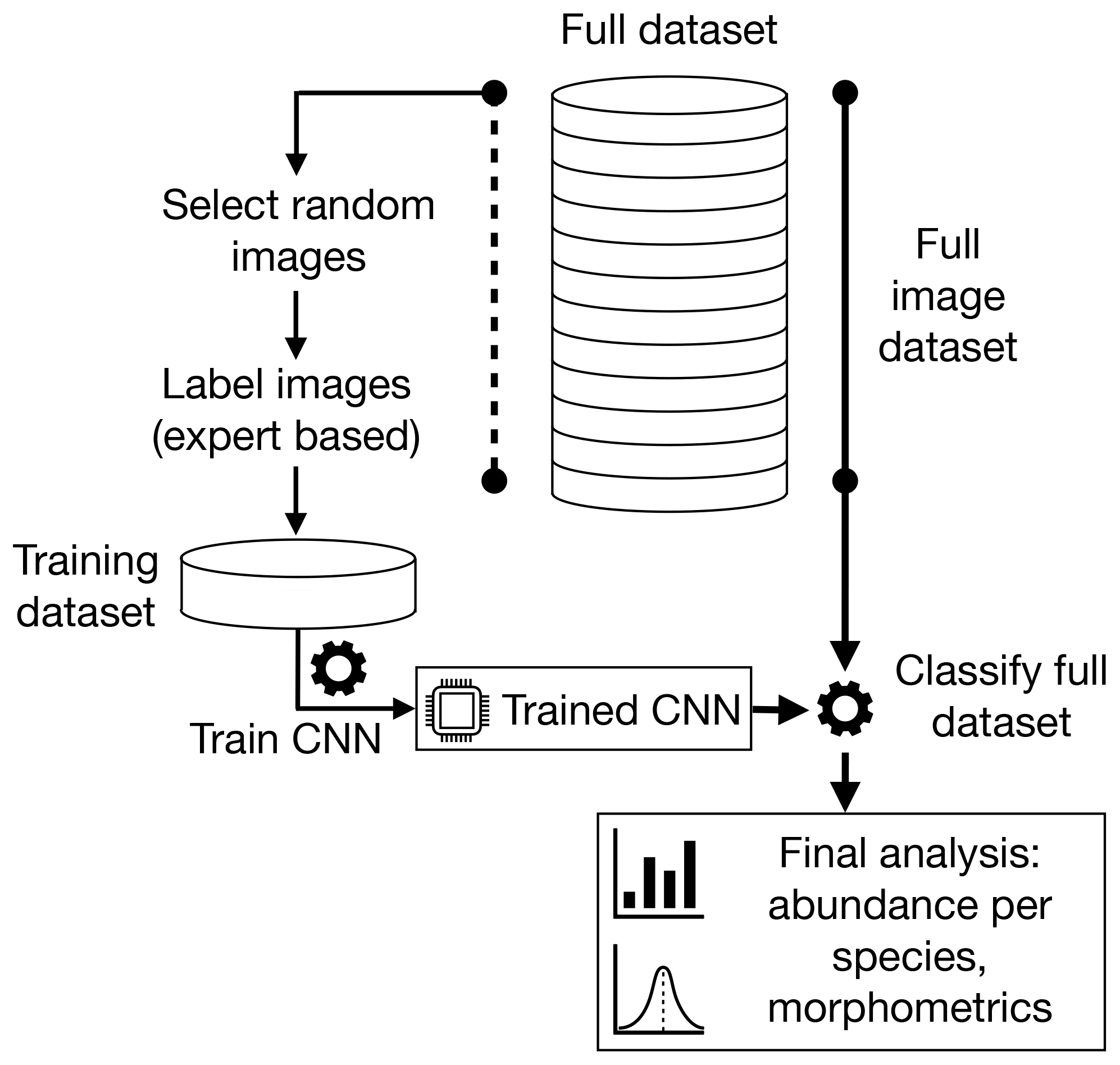
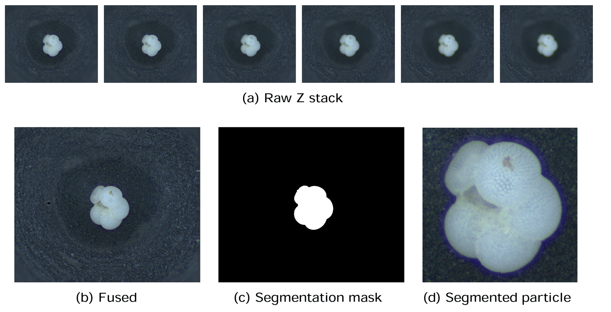
Figure 2The image acquisition process. Raw images form a (a) Z stack which is fused into (b) an in-focus image, from which (c) a segmentation mask is calculated and (d) the foraminifera particle is cropped.
Each foraminifera particle is then cropped into an individual image. Since foraminifera are generally bright white particles, a mask is found using binary segmentation of the image intensity by comparing it to a fixed background threshold – or a dynamic background model in the case of out MiSo machine (Fig. 2c). The mask is smoothed using a morphological opening and then separated into candidate regions of connected pixels. Regions that are too small or too locally concave, thus not representative of a foraminifera shape, are removed. The remaining candidate regions are considered to represent particles. The centre of mass (CoM) and the maximum radius between the CoM and the perimeter are calculated. Each particle is then segmented by cropping a square image centred at the CoM and with side length approximately 2.2 times the maximum radius (Fig. 2d). This ensures the particles appear at roughly the same relative size in the images, with enough of a buffer between the particle and the image border to clearly define its edges. It also ensures that there is enough space to enable rotation of the particle within the image without any parts of the particle clipping the edges of the image. Note that if using images from other sources, e.g. the Endless Forams database (Hsiang et al., 2019), any extra regions with non-photographed information, such as added white regions with metadata text, are removed.
2.2 Training set creation
Supervised training of CNNs involves feeding in batches of images that are labelled with the correct class, typically by a human expert familiar with the domain. The CNN learns to generate the correct label for each image and training is complete when the classification error no longer improves. Curation of the set of training images is therefore important for eventual classification accuracy. The training set should aim to contain all the classes that we expect to encounter in the foraminifera images to be classified. Furthermore, it should cover the intra-class variations that may be present, such as variation in particle appearance caused not only by the natural intraspecific morphological variability and gradation, but also by post mortem effects on the shell such as widely variable preservation figures ranging from dissolution, over-crusts, infillings, damage, fragmentation, etc., to artefacts of sample preparation (residual clays or nano-ooze in poral spaces or in apertures). The training set also has to account for variations in the pose of the particle akin to the aspect, for example umbilical, dorsal or lateral view, rotation in the 2D image plane for a particular aspect, and position and size of the particle in the image. Lastly, the training set has to include any variation within the imaging system, such as brightness, contrast and colour shift, which may be due to camera parameters, lighting brightness, colour and angle, objective distortion or nonuniformity across the field of vision, resolution and detail of the images, artefacts composed of other objects, or background details such as a nonuniform tray surface.
With these caveats in mind, rather than trying to create a single universal foraminifera classifier, we create classifiers (and thus training sets) on a per-core, per-site or, eventually, per-basin basis, akin to regional transfer function schemes (e.g. CLIMAP, 1981). This ensures that the CNN is trained on the species or morphotypes that are specific to that core and that the images are taken using the same acquisition system and camera parameters so that foraminifera specimens are presented with similar luminosity on the same background. As such, a training set is chosen by one of two methods:
-
the first uses images from a few representative samples of the sediment core being analysed or those from similar locations;
-
the second uses a random subset of the images from all the samples in the larger sediment core image set.
Images are then labelled with the aid of the ParticleTrieur software developed at CEREGE. Initially, images are labelled and new classes created as different species or morphotypes are identified. As labelling progresses, the number of images in each class is monitored, and low-count classes are checked to make sure that the spectrum of morphological variability is covered. If there are not enough images in a particular class, more are added to the training set. As a general rule, we aim for at least 200 images in each class, covering all the typical aspects (dorsal, lateral etc.), although it can be difficult to find enough images for some rare classes. Once labelled, the images are exported in JPEG format into directories, one for each class. These form the training image set.
2.3 CNN selection
Once the training set has been labelled, it is used to train a CNN classifier. We use two different CNN topologies:
-
a fast-to-train transfer learning approach that is possible to run on a computer without a high-end graphics processing unit (GPU), and
-
a slower-to-train custom full-depth CNN requiring a computer with a dedicated machine learning GPU that is more accurate and classifies faster.
The transfer learning approach is advantageous to get a baseline estimation of the classification accuracy for each class in the training set. From this, any modifications or additions can be made, for example, checking the labelling or adding more image of a class with low accuracy. Once satisfactory results are obtained, the full-depth CNN is then trained as it is more accurate and classifies faster, meaning that large datasets can be processed more quickly.
2.3.1 Transfer learning
Transfer learning has been employed in other foraminifera classification methods using CNNs, such as in Mitra et al. (2019), Zhong et al. (2018) and Hsiang et al. (2019). Our method takes a slightly different approach in order to speed up training significantly. Firstly, we create a head network, with a ResNet50 (He et al., 2016a) CNN pre-trained on the ImageNet (Deng et al., 2009) database at its core. It consists of a set of transform layers to convert images in the range [0, 1] to the range expected according the preprocessing used in ImageNet pre-training, followed by a cyclic slice layer (Dieleman et al., 2016), then the ResNet50 network with final dense layers removed and replaced with a global average pooling layer, and finally a cyclic pooling layer. Given an image input, the head network outputs a size 2048 feature vector. Secondly, we create a tail network, using the same configuration as Zhong et al. (2018) and Mitra et al. (2019), consisting of a dropout layer (Hinton et al., 2012) with keep probability 0.05, size 512 dense layer, dropout layer with keep probability 0.15, size 512 dense layer and then a final dense layer with softmax activation for the class predictions.
The head network is used to generate a feature vector for every image in the training set. These feature vectors are then used to train the simple two-layer tail network. Because training is restricted to the tail network, only one forward pass through the computationally intensive ResNet50 network is required – when creating the vectors. This means training progresses very quickly. The cyclic layers (Dieleman et al., 2016) are added to give the network some invariance to rotation. Foraminifera images contain many structural features that are repeated at various locations, differing only by their orientation, such as edges at the particle boundary, lines delineating chambers, corners where chambers meet and so on. The cyclic slice layer creates four parallel paths corresponding to rotations of the image of [0, 90, 180, 270∘], while the cyclic pooling layer chooses the maximum response from each of these. In this way, the network is invariant to 90∘ rotations of the image.
After training is complete, the head and tail networks are joined to create a single network suitable for application to images.
2.3.2 Full-depth CNN
We also created a custom compact CNN that adapts to input image size, has only one tuneable parameter and also makes use of cyclic layers. The motivation was that other commonly available topologies are quite large and intensive to train, having been designed with the ImageNet dataset in mind. Our design, called Base-Cyclic, uses convolutional units consisting of a 3 × 3 convolutional layer followed by batch normalization layer and rectified linear activation (ReLU) (Nair and Hinton, 2010). The convolutional layers are initialized using the method of He et al. (2015) as this was found to improve training convergence. Two convolutional units are combined into a block, with a 2×2 max pooling layer at the end. A network consists of N sequential blocks, the number of which, N, is proportional to the input image size according to , which is then rounded to the nearest integer. For example, a CNN for size 128×128 image inputs would use five blocks. The layers in each block have twice the number of filters as the previous block. The output of the final block is flattened and passed into a dropout layer with a keep probability of 0.5. The dropout layer acts to prevent overfitting of the training data (Hinton et al., 2012). Following dropout is a 512-length dense layer with ReLU activation and then the final dense layer with softmax activation and the same dimension as the number of classes.
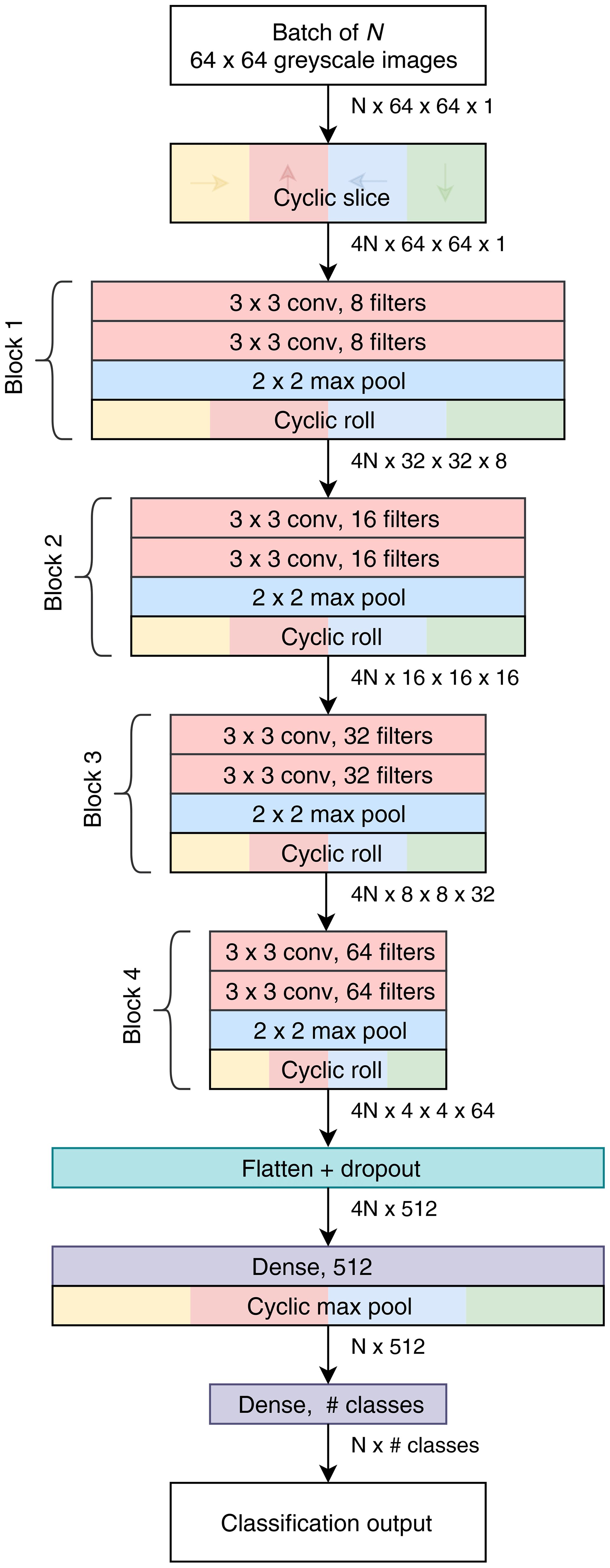
Figure 3Topology of the Base-Cyclic CNN for an input image size of 64 pixels×64 pixels and eight filters in the first block.
A cyclic slice layer is inserted after the image input, and after each convolutional block, the output of each path is rotated back, combined and sliced again (cyclic roll). Then, after the first dense layer, the four paths are combined by choosing the maximum value from each path (cyclic pool). In this type of network, the cyclic layers remove the need for the convolutional layers to learn the same features at multiple orientations and, thus, reduce the number of filters required by 4 times. As a result, we use only eight filters in the first layer.
2.3.3 Input dimensions
A final consideration in the topology is the input dimensions of the images fed to the CNN. As foraminifera can appear at any 2D rotation in a slide image and, thus, have no dominant orientation, we use a square-shaped input. The input dimensions are also determined by the image resolution; using a size greater than the maximum size of the images will require magnification and therefore adds no new information. On the other hand, reducing the input size is useful as it means faster calculations and thus faster training. This may result in an accuracy penalty if important image features needed to discriminate classes, such as pore texture or secondary apertures, are lost.
Unless colour is a discriminating feature in the image set, we prefer to use single channel (greyscale) images where possible, as it removes colour variations that may adversely affect classification, for example when applying the network to another image set with a different colour balance. As a result, for the ResNet50 transfer learning approach, we use greyscale images with size 224×224, while for the Base-Cyclic full network approach we use greyscale images with size 128×128.
2.4 Training
The CNNs are trained using cross-entropy loss on the predicted labels. We randomly select 80 % of the training image set for training, with the remaining 20 % used for validation, and feed the images in batches of 64. Adam (adaptive moment) optimization (Kingma and Ba, 2014) is employed to update the network parameters, using an initial learning rate of 0.001, as this has been found to be good starting point for other image sets (Wilson et al., 2017). Training is performed using code written in the Python programming language and using the TensorFlow v1.14 library (Abadi et al., 2016).
Three parameterless preprocessing steps are applied to the images before training (or inference). (i) The image intensity is rescaled into the range to [0,1], i.e. an 8 bit image is divided by 255 and a 16 bit image by 65 535, which removes variance due to bit depth. (ii) Any non-square images are padded symmetrically to make them square. A constant padding fill value is used, equal to median value of all the pixels lying on the edge of the image. The edge pixels are used because they are normally background pixels due to the foraminifera particle being located in the centre of the image. (iii) The square image is resized to the input dimensions of the network, using bilinear interpolation.
When using full network training, augmentation transforms are applied to images during the training stage to increase the robustness of the CNN (e.g. Simard et al., 2003) to image variations. We apply augmentation to simulate some of the variances that arise from the foraminifera imaging system; it is performed in parallel on a GPU during training and does not noticeably increase training time. An augmented image, is created from the original image I using the following transformations:
-
a random rotation between 0 and 360∘;
-
a random gain (β; brightness) chosen from applied using the formula ;
-
a random gamma (γ; contrast) chosen from applied using the formula . This requires the input images to be in the range [0,1];
-
a random zoom chosen from . Values above 1.1 are not use as they would clip the particle in the image.
The training loss function is also weighted inversely according to the count of images in each class. This is to ensure the CNNs do not overfit on the classes with more numerous examples and to boost the accuracy on the more rare foraminifera that may not be very abundant. The weighting per class is given by the geometric mean of all the class counts divided by the individual class count:
where wi is the weight for class i, and ki is the class count. The weight values are clamped at a minimum of 0.1 and maximum of 10 so that the range of values is not too extreme.
We employ a periodic decrease in learning rate as this tends to increase classification accuracy (e.g. He et al., 2016b). An automated method is used to scheduling learning rate drops and stop training, as this removes the need to tune the number of training iterations. The method is based on the approach used in the dlib library (King, 2009). The loss, yi, after each training batch xi in the last n batches, with index , is modelled as a linear function with the slope, m, and intercept, c, corrupted by Gaussian noise, ϵ:
The slope of the noisy loss signal of the last n values is a Gaussian random variable with the distribution
where
The probability, P, of the true slope (m) being below 0, which indicates that the training score is improving, is given by the Gaussian cumulative distribution function:
where is found using a linear regression over .
After each batch, we calculate P; if P<0.51, we assume that training is no longer improving and drop the learning rate by half. Calculation of P is then paused until another n batches have been processed. This process is repeated a specified number of times (drops) after which training is stopped. We express the number of batches in terms of number of epochs (complete run through the training set):
where L is the number of epochs. Thus, changing the size of a batch does not affect the actual number of images considered when calculating P. The number of epochs and drops are tuned to the training set, and we find that those with large numbers of images per class require fewer epochs. For smaller training sets (<5000 images with fewer examples per class), we use 40 epochs and four drops. For larger sets, the number of epochs is reduced (e.g. 10 epochs for > 10 000 images). More drops are added if the noise in the validation accuracy is still significant after four drops. Henceforth, we refer to our automatic learning rate scheduler as ALRS.
At the end of training, the network is “frozen”, whereby trainable variables are replaced with constants and saved in protobuf format. An XML file is created with metadata about the network, such as the input size and class names, so that all the information necessary to be able to use the network for classification is present; thus, the CNN can be readily shared with other users. Note that an optional step is to train the entire image set (both training and validation) on the best-performing network. Since there are no validation images the accuracy cannot be measured; however, one would expect that the extra images should improve classification performance on new images.
2.5 Evaluation
The remaining random 20 % subset of training data is used to validate the performance of the trained CNN. We calculate the following classical measures.
-
Overall accuracy – the percentage of images in the validation set that were correctly classified by the CNN; higher accuracy means better classification performance; we also calculate some per-class measures and report them averaged over all classes.
- –
Precision: the percentage of images identified into a class that actually belong to the class;
- –
Recall: the percentage of images in a class that were correctly identified (per-class accuracy); and
- –
F1 score: the average of precision and recall.
- –
-
Training time – the time to train the network, including feature vector calculation in the case of transfer learning; a long training time can reduce the efficiency of the workflow, especially during a hyper-parameter search where training is performed multiple times; networks with very short training times may be possible to train on a computer without a GPU;
-
Inference time – the time to classify a single image; longer inference time means longer to classify large image sets.
2.6 Classification
Finally, the chosen trained network is used to classify the larger image set. The images are arranged into folders by depth. Each is preprocessed as for training (Sect. 2.1) and passed through the CNN to calculate the softmax output of the final layer. The output is a vector of prediction scores, one for each class, ranging from 0 to 1, with all scores adding to one. We consider a score above a fixed threshold as a positive classification for the class. If no scores are above the threshold, the image is classed as “unsure”. The threshold must be chosen from the range (0.5, 1.0] as then only one class will be above the value. We use a threshold of 0.8.
3.1 Ablation study on Endless Forams
An ablation study was performed to investigate different CNN topologies and their parameters for foraminifera classification, using the large, publicly available Endless Forams core-top planktonic foraminifera image set (Hsiang et al., 2019). All images of this database have been congruently assigned to one species by a set of independent taxonomists, providing a unique benchmark for recent planktonic foraminifera. The image set consists of 27 729 colour images in 35 species classes, ranging from four specimens (Globigerinella adamsi) to 5914 specimens (Globigerinoides ruber) in each class. We excluded five classes, Globigerinella adamsi (4), Globigerinita uvula (7), Tenuitella iota (8), Hastigerina pelagica (13) and Globorotalia ungulata (25) because they had less than 40 images, meaning that only one to eight images are available for validation and, thus, are likely not reliable measurements. Each image was preprocessed to remove the white metadata panel at the bottom of the image and the black border around the particle, so that only the real photographic part of the image remained, then padded to make them square using the method outlined in Sect. 2.1. The processed images are available for download from https://github.com/microfossil/datasets-and-models (last access: 2 October 2020).
Both the transfer learning (Sect. 2.3.1) and full network training (Sect. 2.3.2) approaches were investigated. Training was run using TensorFlow 1.14 and Python 3.7, on a Windows 10 desktop computer with NVIDIA RTX 2080 Ti GPU, AMD Ryzen 2700X CPU, Sandisk 970 EVO SSD and 32 GB of RAM.
3.1.1 Transfer learning
A first experiment was performed on the choice of network to use as the core of the transfer learning method (Sect. 2.3.1), excluding the cyclic layers. Colour images at the default size for each network (224×224 except for 299×299 for Xception and NASNet) were used, and 10 epochs and four drops were set for the ALRS. Training was repeated five times using 5-fold cross validation, and each performance measure was averaged across the set. The ResNet50 network outperformed all other networks for accuracy (81.8 %) and took only 198 s to train. MobileNetV2 was the fastest to train, thanks to having the fastest inference time (1.25 ms compared to 2.11 ms for ResNet50), which makes precalculating the feature vectors faster (Table 1).
Table 1Results of training various transfer learning networks on the Endless Forams training set (colour images). Training time includes precalculation of the feature vectors. a images, b images. Best performance for each measure is shown in bold.
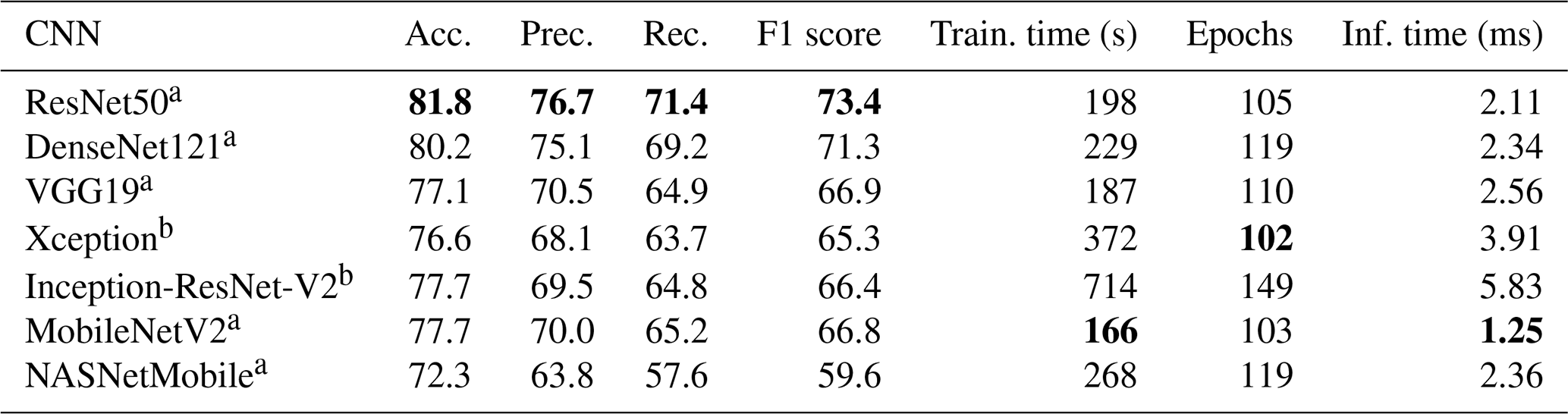
Table 2Results of training on the Endless Forams training set (colour) using the best-performing transfer learning network with and without cyclic layers – and for different input image sizes. Best performance for each measure is shown in bold.
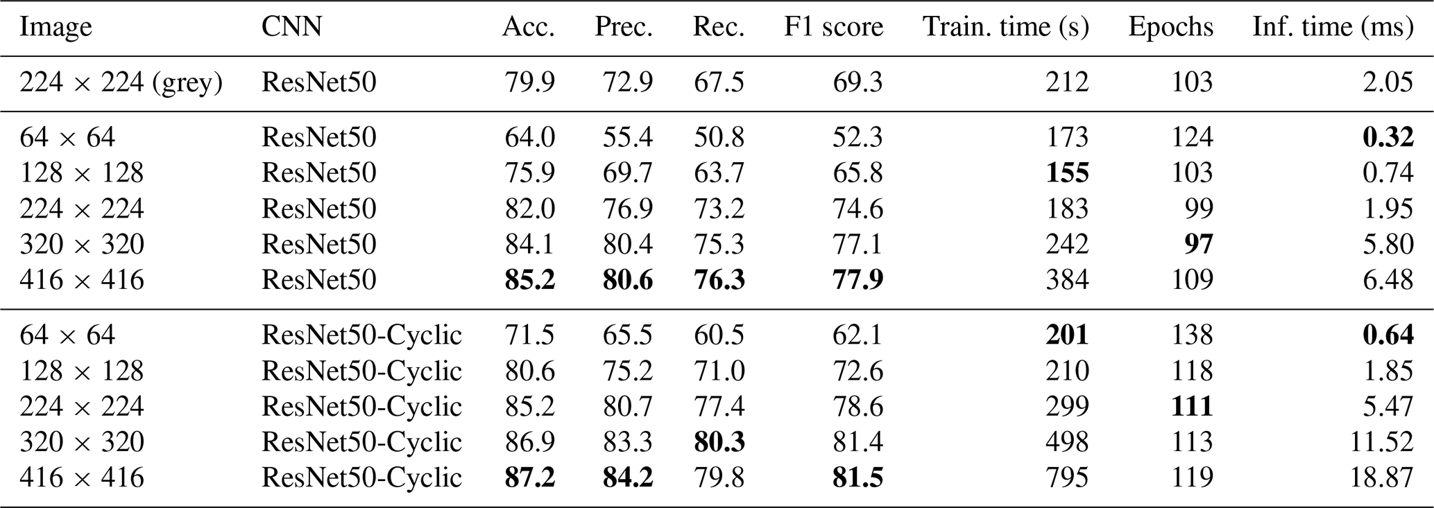
Given that ResNet50 had greatest accuracy, we explored the effect of image size and cyclic layers on this topology (Table 2). Initially, greyscale images were used; however, this reduced the accuracy to 79.9 %, so colour images were used for the rest of the comparison. It is likely that the reduction in performance was because colour is an important discriminating factor for some of the images in this dataset, perhaps due to seemingly different image acquisition settings being used for some of the classes. Interestingly, increasing the image size improved accuracy, up to 85.2 % for 416×416 images. However, this significantly increased memory requirements, with the training set (represented as 16 bit floating point numbers) using approximately 28 GB of memory. The inference time also increased with the image size, taking more than 3 times longer to process 416×416 images (6.48 ms) than 224×224 images (1.95 ms). Using cyclic layers improved the accuracy by between 2 % and 6 % for all image sizes, with a maximum accuracy of 87.2 % for 416×416 images. However, the improvement came at the expense of the inference time, which more than doubled. Using cyclic layers is a simple technique to improve all types of transfer learning where the feature vectors are precalculated.
3.1.2 Full network
We also compared full network training of the commonly available ResNet18 network with our custom Base-Cyclic network as well as a variation of this called ResNet-Cyclic where the two-layer convolution blocks were replaced with ResNet blocks with skip connections. Image sizes of 64×64 and 128×128 greyscale images were used for the comparison. For our custom networks, the number of filters in the first block was varied between 4 and 16 (Sect. 3).
For both 64×64 and 128×128 images, the Base-Cyclic design with 16 filters gave the best overall accuracy of 87.5 %, whereas the ResNet-Cyclic design with 16 filters gave the best class-averaged precision and recall. In all cases, using 128×128 images gave higher accuracy, up to 90.3 %. The training time increased proportionally with image size and the number of filters, and the ResNet-Cyclic network took longer than the Base-Cyclic network (up to almost 3.5 h for one configuration). The long training time is why larger image sizes were not investigated further; however, it may be feasible for smaller sets of just a few thousand images. The inference time was low for all configurations, ranging from 0.09 to 0.68 ms, except for the standard ResNet18 network with was 2.05 ms. We use the Base-Cyclic network with eight filters in our workflow, as it provides a faster training time with only a small (0.2 % for this dataset) decrease in accuracy compared with 16 filters.
Table 3Results of full network training on the Endless Forams training set (greyscale) for different input sizes and number of filters. Best performance for each measure is shown in bold.
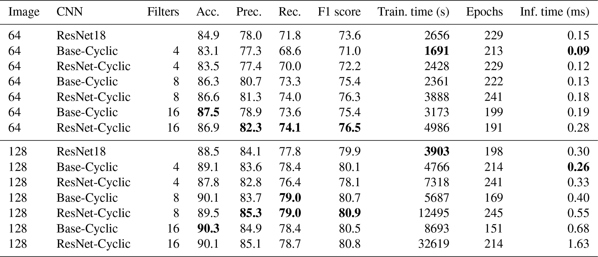
The full network training gave better accuracy than the transfer learning methods at the expense of much longer training times; however, the inference times of the transfer learning networks were around 2 to 10 times longer than the largest Base-Cyclic full network. Therefore, despite their long training times, the shorter inference times and higher accuracy of the Base-Cyclic and ResNet-Cyclic design make them more suitable for processing large image sets. Each of the networks ResNet18, Base-Cyclic and ResNet-Cyclic gave higher accuracy than the VGG16-based networks used by Hsiang et al. (2019), with a maximum of 90.3 % (Base-Cyclic with 16 filters), which is almost 3 % more than their reported maximum of 87.4 %.
3.2 Application to benthic foraminifera dataset (core MD02-2508)
We applied our method to create a high-resolution analysis of the Holocene interval within sediment core MD02-2508, retrieved from the north-eastern Pacific oxygen minimum zone during the R/V Marion-Dufresne MD126 MONA (Image VII) campaign in 2002 (Beaufort, 2002).
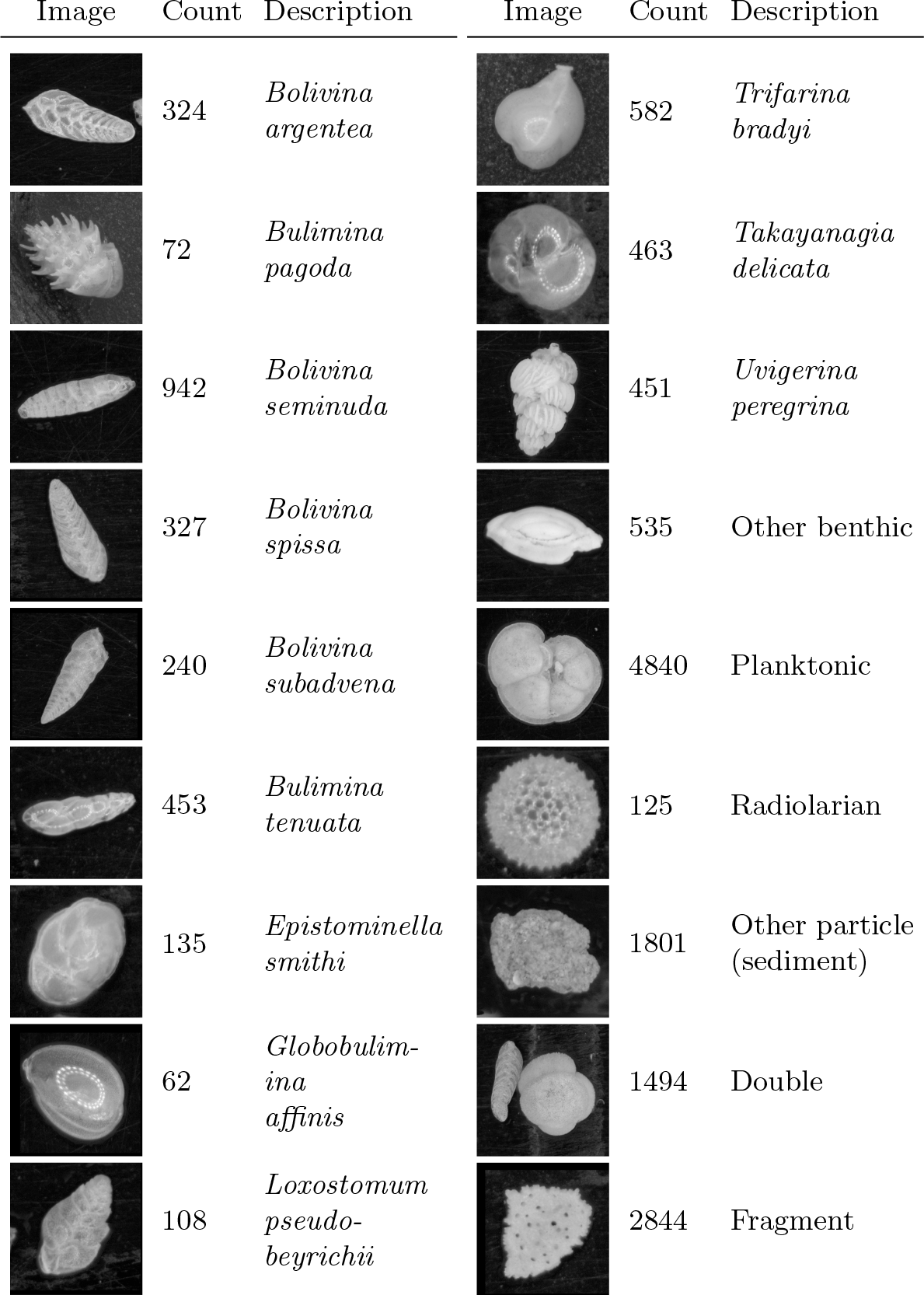
Figure 4Example image from each class of training set constructed from cores MD02-2508 and MD02-2519, classified mainly by species. There are 15 274 images in total.
3.2.1 MD02-2508 sediment core dataset
A large image set (73 544 images) was acquired for core MD02-2508 using the imaging system described in Sect. 2. Some images were taken with the particles on a micropalaeontological slide, and some images were taken using the MiSo particle sorting machine at CEREGE. Individual particles were segmented from these larger images as per our method. Images were taken of 41 samples from 40 to 642 cm deep. These samples were chosen to cover the Holocene and the deglaciation (0–16 000 years ago) as given by the age model for this core (see Tetard et al., 2017). Manual counting of benthic species in the core had already been performed for 37 samples in this depth range (Tetard et al., 2017) and were used for comparison.
3.2.2 MD02-2508 training set
A training set was constructed from 15 274 images of foraminifera from seven representative samples from cores MD02-2508 and MD02-2519. The images from MD02-2519 (not the core of interest) were used, as this core is from a similar location to MD02-2508, contains a very similar benthic foraminiferal fauna and the images had already been acquired. The training images were manually labelled using the ParticleTrieur software into 12 benthic species (main species according to Tetard et al., 2017), an “other-benthic” class (grouping the less abundant benthic species), a single catch-all planktonic class, a radiolarian class, and some non-foraminifera classes such as “double” (specimens in contact with each other) and fragments (Fig. 4). Images ranged from 188 pixels×188 pixels to 1502 pixels×1502 pixels in size, corresponding to particles 140 to 1100 µm in diameter.
3.2.3 MD02-2508 classification
The images were used to train a Base-Cyclic network with eight filters, using 10 epochs and four drops for the ALRS system. We obtained an overall accuracy of 89 % with most classes having above 75 % accuracy. There was some confusion between similar looking Bolivina benthic species, B. spissa, B. subadvena and B. seminuda. Precision and recall (per-class accuracy) tended to be higher for those classes with a high count in the training set, and almost all classes had some confusion with the fragment class (Fig. 5).

Figure 5Confusion matrix of one training run on the core MD02-2508 training set. After training, each image in the validation set is classified with the CNN and compared to the true classification. Each cell shows the percentage of images in the class on the left (row labels) that were classified into the class on the bottom (column labels), for the validation set. Perfect classification would result in 100 % along the diagonal axis, whereas nonzero values off the diagonal mean that the class on the left was confused with the class on the bottom. The number of images in the validation set for each class is shown in brackets next to the class label (total number in the training set is 5 times this amount).
A review of the training set found errors such as mislabelling and duplicate images (due to a slight overlap in the images acquired using an automated stage) that were labelled into different classes, and these may have negatively affected the accuracy. Furthermore, the presence of plastic core liner or sediment particles touching the foraminifera of interest occasionally resulted in the image being classified into either the double class or another class with similar shape to their combined appearance. Likewise, the variability in fragmentation from slight damage to a single chamber to larger damage affecting a number of chambers may explain why some images in each class were classified as fragments (Fig. 5).
3.2.4 MD02-2508 class abundance
Manual counting of samples from MD02-2508 had previously been performed for every benthic species recovered from this core. For the results of both manual and CNN counting, we separated out eight of the main species that are of interest for palaeoceanographic reconstructions (Tetard et al., 2017) and placed the rest into an other benthic class. The relative abundance was then calculated for each benthic group compared to the total benthic count, for each method. Since the planktonic classes were undifferentiated, and no manual counting had been performed for them, we instead calculated the percentage of benthic foraminifera to whole foraminifera (planktonic + benthic) from the CNN counts over the same period and compared the dynamics of this signal to the Greenland oxygen isotopic record, an indicator of Northern Hemisphere climatic changes.

Figure 6Relative abundance of eight benthic species in core MD02-2508 (top) both human (blue squares) and automated (red circles), image counts per sample in the automated system (bottom left) and the benthic foraminifera to whole foraminifera ratio from automated counting compared to the Greenland oxygen isotopic record (bottom right).
The signals obtained using CNN classification had similar dynamic characteristics to those from manual counting (Fig. 6).
-
Counts for Bolivina argentea are higher than for the human counts in the more recent samples; however, the signal exhibits the same dynamics, with the same peaks in abundance around 10 000, 3500 and 1200 a BP.
-
B. seminuda also shows similar abundance to the human counts, with gradually increasing abundance towards the modern day. The short spike in abundance around 7500 a BP is also visible.
-
Human counting of B. spissa is zero for the Holocene, and this species is usually absent from this area during this period. The CNN finds some 5 % of specimens as B. spissa, suggesting all of these images may have been misclassified.
-
Counts of B. subadvena show similar absolute abundance and dynamics as human counting, except for a peak around 6500 a BP.
-
Buliminella tenuata shows the same large peaks at 11 500 and 14 000 a BP. The transition from almost zero abundance at 9500 a BP to above 30 % abundance at 11 500 a BP is also much smoother for the CNN-derived results, suggesting that the larger number of images processed result in less noise for the highly abundant species.
-
Human counts for Epistominella smithi during the Holocene are zero, suggesting the absence of this species during this time in this particular area. The CNN counts are also low during this period, in contrast to the B. spissa signal.
-
Similarly, the nonzero CNN counts of Uvigerina peregrina during the Holocene are likely due to the presence of a morphologically close species: U. striata, present in the other benthic class.
-
The CNN signal for Takayanagia delicata also follows the human counting, with a peak at 11 500 a BP present in both results.
-
Both human and CNN abundances show other benthic species at around 10 % during the Holocene and 20 % before it. The CNN counts are much smoother.
-
CNN counts show that the percentage of benthic foraminifera was very high during the Holocene, dropping off around 11 500 a BP. The dynamics of the signal very closely match that of the Greenland oxygen isotopic record, correlating with other studies that show that benthic foraminifera abundance and marine productivity were higher during warm periods (especially the Holocene) in this area (Cartapanis et al., 2011, 2014; Tetard et al., 2017). The results also indicate that the CNN can successfully discriminate benthic from planktonic species, likely due to the greater difference in morphology compared to within-benthic species differences.
3.3 Application to planktonic foraminifera dataset (core MD97-2138)
The method was also applied to planktonic foraminifera to create a high-resolution analysis of the last climatic cycle within sediment core MD97-2138, retrieved from the western Pacific during the IPHIS cruise in 1997 on the R/V Marion-Dufresne (Beaufort, 1997; de Garidel‐Thoron et al., 2007).
3.3.1 MD97-2138 sediment core dataset
A very large image set (562 363 images) was acquired for core MD97-2138 using the imaging system described in Sect. 2. All images were taken using the MiSo particle sorting machine at CEREGE, and individual particles were segmented from these larger images as per our method. Images were taken of 49 samples from 1 to 945 cm deep, with an average of 11 477 particles (foraminifera, aggregate, etc.) imaged per sample. These samples were chosen to cover the whole last climatic cycle, from the Holocene to Marine Isotope Stage 6, as given by the age model for this core. Manual counting of planktonic species in this core had already been performed for 123 samples in the same depth range, averaging 342 specimens identified per sample, and counting of fragmented and whole foraminifera for 99 samples, averaging 568 per sample (de Garidel‐Thoron et al., 2007).
3.3.2 MD97-2138 training set
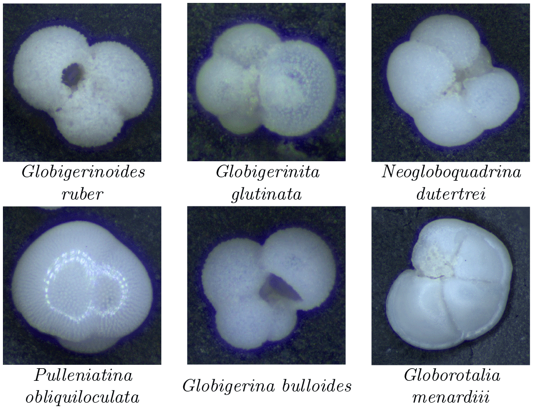
A training set was constructed from 13 001 images of particles randomly selected from the larger MD97-2138 dataset that was to be classified. The same taxonomy (35 species classes) as used in the Endless Forams dataset was used to label the images, with the addition of five extra classes (aggregate, background, benthics, double and fragment) to cover additional images that did not fit into one of the planktonic species classes. To speed up the labelling process, the training set was pre-labelled using the best-performing CNN trained on the Endless Forams set from Sect. 3.1 and manually checked and corrected where necessary. Images ranged from 171 pixels×171 pixels to approximately 2000 pixels×2000 pixels in size, corresponding to particles 140 to 1500 µm in diameter, with a median of 310 µm.
3.3.3 MD97-2138 classification
The images were used to train a Base-Cyclic network with the same configuration as for the benthic set. Again, classes with less than 40 specimens were dropped from the training set, giving a total of 20 classes. An overall accuracy of 90.7 % was obtained, with those classes containing numerous images generally giving better accuracy (Fig. 8). Of the classes with less than 500 images, surprisingly, the simplest planktonic species Orbulina universa (spherical chamber; 95 images) had among the worst recognition rate with only 47.4 % recall, due to being confused with fragments. The network had difficulties in learning the subtle difference between a large broken chamber of G. siphonifera, for example, and O. universa. The species with the worst performance was Neogloboquadrina incompta with a recall of 39.3 %; however, most of the false negatives were classified as N. dutertrei (54 %), which belongs to the same genus and to the same Pachyderma–Dutertrei (P-D) intergrade. As with the benthic set, almost all classes had some confusion with the fragment class.
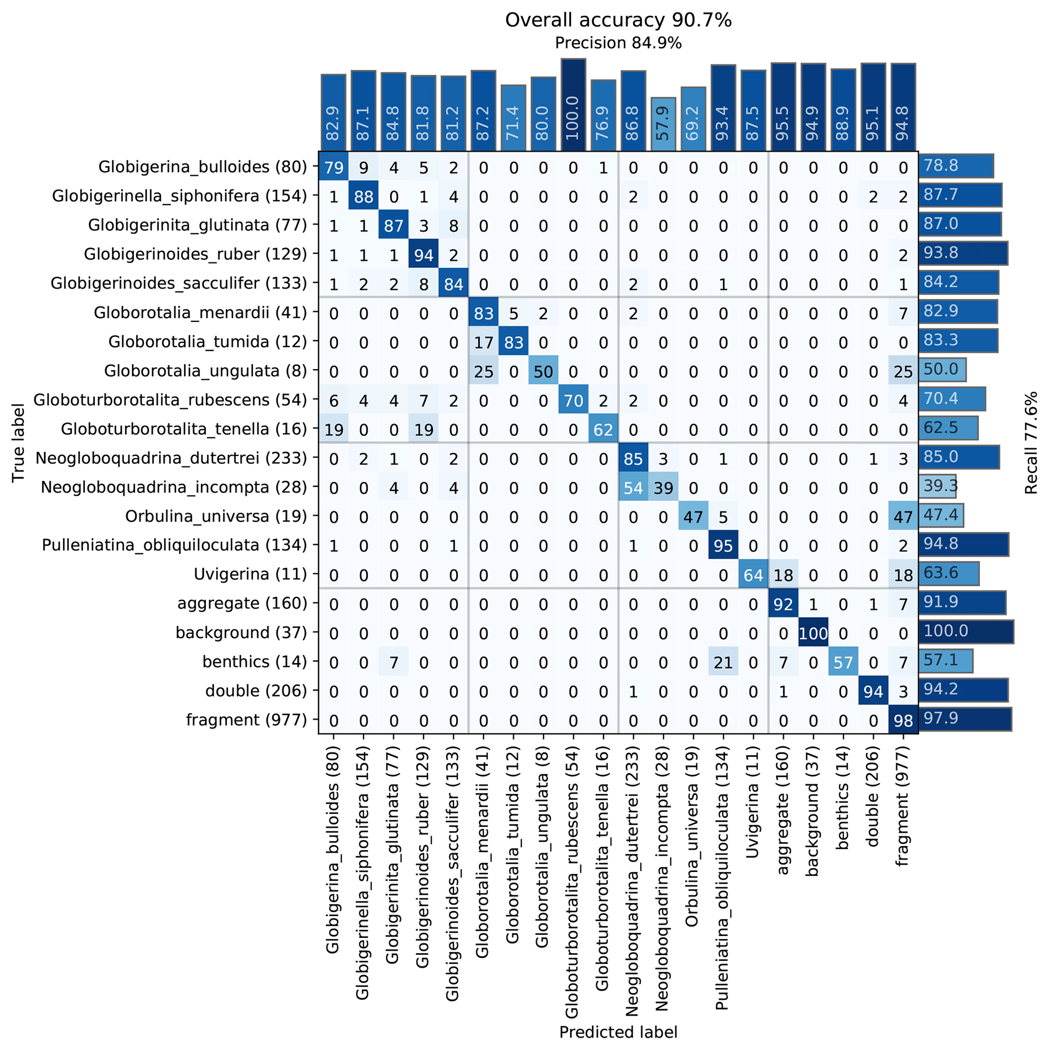
Figure 8Confusion matrix of one training run on the core MD97-2138 training set. After training, each image in the validation set is classified with the CNN and compared to the true classification. Each cell shows the percentage of images in the class on the left (row labels) that were classified into the class on the bottom (column labels), for the validation set. Perfect classification would result in 100 % along the diagonal axis, whereas nonzero values off the diagonal mean that the class on the left was confused with the class on the bottom. The number of images in the validation set for each class is shown in brackets next to the class label (total number in the training set is 5 times this amount).
3.3.4 MD97-2138 class abundance
Manual counting of planktonic species and fragmented shells had previously been performed for samples from MD97-2138 (de Garidel‐Thoron et al., 2007). To compare the results of both manual and CNN counting, we separated out the six most common species and calculated the relative abundance compared to all planktonic foraminifera, as well as the percentage of fragmented particles to all foraminiferal particles, for both methods. The number of images analysed using the CNN approach typically exceeds 2000 images and reaches more than 18 000 compared with the typical 300–350 foraminifera usually counted by a human taxonomist. We also calculated the abundance using automatic counting with a CNN trained on the Endless Forams dataset.

Figure 9Relative abundance of the six most common planktonic species in core MD97-2138 (top) for both human (blue squares) and our automated system trained on the core-specific training set (red circles) or Endless Forams dataset (green diamonds), image counts per sample for the automated system (bottom left), and the percentage of fragmented particles out of all foraminifera particles (bottom right).
The signals obtained using both the Endless Forams network and the MD97-2138 CNN network classification show similar dynamic characteristics to those from manual counting (Fig. 9) but with more consistency in results from sample to sample. The CNN trained on MD97-2138 images always gives results closer to the human count, whereas the Endless Forams-trained classifier systematically underestimates the percentage of those main species. However, the general trends are similar when comparing the Endless Forams and MD97-2138 networks. We focus now on the comparison of the MD97-2138 CNN classifications with the human classifications.
-
Counts for G. ruber are consistently within the same range as the human counts, with the same counts from the recent data and a dip between 60 000 and 110 000 a BP.
-
Globigerinita glutina is slightly underestimated compared with human counting.
-
There is a close alignment of N. dutertrei with a peak at 15 000 a BP that matches the human counts.
-
Pulleniatina obliquiloculata also matches human counts; however, the CNN abundance does not exhibit the same three-peak structure during the previous interglacial.
-
Counts for Globigerina bulloides are consistently lower (by 5 % to 10 %) for the CNN counts compared with the human counts.
-
Globorotalia menardii is not as abundant as the other species, but the signal appears to match for each method.
-
The fragmentation rate between both CNN counting and human counting match almost perfectly, albeit with a smoother signal for the CNN counts.
4.1 Benthic foraminifera dataset (core MD02-2508)
The dynamics of each abundance signal calculated for the benthic foraminifera dataset using our automated CNN method were similar to that obtained from manual counting. However, we noticed that the strongest bias in most species is likely caused by false positives. The misclassified images were inspected to find the source of the errors, and as with the training results for this dataset, the various species of the Bolivina genus were generally confused with each other. In particular, many specimens of B. subadvena were misclassified as B. spissa, causing the nonzero counts for this species during the Holocene.
One possible explanation is that the intraspecific morphometric variability for species B. argentea, B. spissa and B. subadvena can be higher than the interspecific variability between these species. For example, the microspheric forms of different species can appear more similar to each other than with the microspheric and macrospheric forms of the same species. As a consequence, the identification and discrimination of these forms can be difficult even for a taxonomist, and the CNN also mistakes these species more often. This can also explain why E. smithi, which was also not present in the core during the Holocene, did not have a strong false positive bias, as few other classes were confused with it during training.
We note some species can be discriminated under a stereoscopic microscope by their flatness, (e.g. B. spissa and B. argentea versus B. subadvena and B. seminuda), which helps for manual identification, but this depth information is lost for the 2D images in our automated approach. Thus, this bias is largely dataset dependant, as four of the eight main species analysed in this study belonged to the same genus (i.e. Bolivina). Hence, the dataset provides a good case study on the performance of a CNN classifier; overall, most of the classes were correctly identified.
4.2 Planktonic foraminifera dataset (core MD97-2138)
As for the benthic dataset, the dynamics of each abundance signal calculated for the planktonic dataset using out method were similar to those from manual counting. The two main discrepancies in the abundance records are the significant underestimation of G. bulloides and some poor recognition in the highest peaks of P. obliquiloculata. With regards to the underestimation (by 5 % to 10 %) of G. bulloides, the dataset does include a lot of images of foraminifera whose umbilical aperture is not fully cleaned and is infilled with remaining nannofossil ooze. Such infilling often precludes the CNN from classifying these image correctly. The other factor that might explain this underestimation is that the G. bulloides in the western Pacific warm pool are smaller and not as well imaged as the larger species investigated here.
The second striking diverging feature is the lack of peaks in the abundance signal for P. obliquiloculata. We interpret this to be caused by some aliasing in our automatic approach that is not as well resolved during the Marine Isotopic Stage 5 as the human counts were and is likely a result of the strong dissolution affecting those intervals, as seen in the fragmentation records. However, apart from those two main exceptions, the general automated population changes are quite close to those derived by a micropalaeontologist and allow this method to be fully implemented for palaeoceanographic reconstructions. Such automated reconstructions based on images have already been widely used for coccoliths (e.g. Beaufort et al., 2001) but not yet for foraminifera at the species level. This approach also allows for the detection of the appearance or disappearance of species for biostratigraphical studies. Our study, due to its short time span (less than 150 kyr), cannot fully test this approach, with the only major datum being the disappearance of G. ruber pink at 130 kyr BP (Thompson et al., 1979); moreover, our CNN was not trained on colour images.
The CNN trained on the Endless Forams dataset gave similar accuracy to the CNN trained on the MD97-2138 dataset for G. ruber; however, for other species it did not estimate the abundance well. This failure to generalize is possibly due to the different imaging conditions and different species present int the set. It reinforces our approach of randomly sampling the full dataset to create the classification training set, as this ensures the same distribution of morphometric variation in the images to be classified, and also the same range of taphonomical biases (dissolution, etc).
In this article we have presented a method for analysing large foraminifera image sets using deep convolutional neural networks. The performance of transfer learning and full network training for publicly available CNNs, as well as our custom Base-Cyclic and ResNet-Cyclic designs, were demonstrated on the Endless Forams image set, as well as our core-specific benthic and planktonic training sets. The transfer learning approach is fast to train and gives good accuracy without augmentation. Full network training is much slower to train, but our Base-Cyclic design gives as good or better accuracy with faster inference time. Our approach has been to use transfer learning when a CNN is needed quickly to aid with manual labelling and to use full network training to create the final network used for analysis of the entire dataset.
This method of automatic identification is routinely used at the CEREGE laboratory, in combination with the high-throughput imaging and sorting machine, MiSo. Our workflow can also be applied to classify other images of bio-indicators, such as radiolaria, coccoliths, pollen or plankton. An important observation we have made is the sensitivity of CNN accuracy to imaging set-ups: even with heavy image augmentation, classifying images using a CNN trained on images from a different acquisition system is not as accurate as classifying with those trained on image obtained from the same system. In particular, a change in background can cause gross misclassification, e.g. a particle imaged on a micropalaeontological tray compared to one imaged in our MiSo foraminifera sorting machine. We recommend keeping the same imaging settings for both the overall sediment core image set and the training image set.
Likewise, one should optimize the training set according to the sediment or core under analysis. This is important in three ways: the training set should (i) incorporate all the main taxa and their morphological variants; (ii) have undergone the same early diagenetic history, to ensure that the range of dissolution, early pyritization (which can affect structure), colour, and translucency are included in the morphological variability; and (iii) include non-foraminifera artefacts that could affect classification, such as particles (e.g. plastic core liner or sediment) or specifics of the acquisition system (e.g. ring light pattern). In our method, we choose a random subset of the larger image set under consideration to create the training set, as the random sampling should capture this variability and thus make the final classification more robust.
One limitation of the method described here is that each foraminifera specimen is only represented by a single hyperfocal image at classification time. Species that require multiple views to make a clear distinction are therefore less likely to be correctly identified. Another drawback is that foraminifera are placed onto slides by dropping them randomly. Many species appear to have a preferential pose, but some may land in orientations where distinguishing features are not visible. Rectifying either of these problems would require a change to the imaging system to support multiple views, at the expense of increased processing time. We also note that information about the foraminifera size is lost when the images are processed to a uniform dimension for presentation to the CNN, this detail may be important for discriminating some species who are more easily recognized by their size. Furthermore, our CNN typically does not use colour images so that the effect of variations in lighting are minimized. However, this prevents the identification of some species such as G. ruber pink or G. rubescens.
The example applications on analysing benthic foraminifera in one core and planktonic in another show that a very large throughput is possible with an automated system. Indeed, over 0.5 million specimens were processed for the planktonic core. In this way, a few hours labelling a well-constructed training set saves months of time manually counting specimens. Furthermore, the CNN obtained can be repurposed to aid in constructing other training sets by using the predictions to suggest labels, as we did when constructing the planktonic training set using a CNN trained on Endless Forams. One of the major advantages of this approach is the possibility to routinely combine counts and morphometric analyses at the species level, a novelty for the analysis of foraminifera whose morphometric analyses in sediment cores are usually based either on a singular species or a combination of all specimens regardless of species. Chamber delineations as described by Ge et al. (2018) are also achievable with a good imaging system, and it would be very helpful to complement CT-scan analyses on a limited number of specimens (e.g. Caromel et al., 2015). Those applications are all in reach given the described workflow can acquire and process around 10 000 images per day.
Morphometric information that is not well represented by a CNN could assist in foraminifera classification, for example, chamber count and texture distribution. Although this requires feature engineering rather than learning, the measurements are interpretable and thus relevant to taxonomists and rule-based classification, where CNN features which are local are generally not interpretable and not necessarily consistent between image sets. Likewise, specimen thickness could help discriminate round and flat species, such as B. spissa and B. subadvena in the benthic image set. Thickness can be estimated from the depth map calculated when performing multi-focal image fusion. In future work we propose to combine images with morphometric features and depth map information in a new CNN-based classification system.
The ParticleTrieur software program, which was used to manually label the training set and automatically classify foraminifera images, is available with tutorials from http://particle-classification.readthedocs.io (Marchant, 2020a). The latest version of the Python scripts (https://doi.org/10.5281/zenodo.3996358, Marchant, 2020b) to train the CNNs in this paper are available from http://www.github.com/microfossil/particle-classification (last access: 2 October 2020) and can be installed using the “pip” Python package. The Endless Forams (Hsiang et al., 2019), MD022508 and MD972138 training sets (https://doi.org/10.5281/zenodo.3996436, Marchant et al., 2020) are available from https://github.com/microfossil/datasets-and-models (last access: 2 October 2020).
RM developed the system, performed the experiments, acquired images for core MD02-2508 and was the primary author of the paper; MT acquired and expertly labelled the images for core MD02-2508 and edited the paper; AP acquired and labelled the images for core MD02-2508; MA and TdGT labelled the images for MD97-2138; and TdGT organized the project and its funding and also wrote the publication.
The authors declare that they have no conflict of interest.
This work was funded by the Agence Nationale de la Recherche FIRST project (ANR-15-CE4-0006-01). The research leading to these results has received funding from the People Programme (Marie Curie Actions) of the European Commission's Seventh Framework Programme (FP7/2007-2013) under REA grant agreement no. PCOFUND-GA-2013-609102, through the Prestige Programme coordinated by Campus France. We thank Yves Gally for his help in setting the computer in the automated microscopy laboratory, Jean-Charles Mazur and Sandrine Conrod for sample preparation, and ATG Technologies for the joint design of the automated system.
This research has been supported by the Agence Nationale de la Recherche (grant no. ANR-15-CE4-000601), the Seventh Framework Programme (PRESTIGE; grant no. PCOFUND-GA-2013-609102) and ECCOREV Rapp project.
This paper was edited by Sev Kender and reviewed by Mike Simmons and Marit-Solveig Seidenkrantz.
Abadi, M., Agarwal, A., Barham, P., Brevdo, E., Chen, Z., Citro, C., Corrado, G. S., Davis, A., Dean, J., Devin, M., Ghemawat, S., Goodfellow, I., Harp, A., Irving, G., Isard, M., Jia, Y., Jozefowicz, R., Kaiser, L., Kudlur, M., Levenberg, J., Mane, D., Monga, R., Moore, S., Murray, D., Olah, C., Schuster, M., Shlens, J., Steiner, B., Sutskever, I., Talwar, K., Tucker, P., Vanhoucke, V., Vasudevan, V., Viegas, F., Vinyals, O., Warden, P., Wattenberg, M., Wicke, M., Yu, Y., and Zheng, X.: TensorFlow: Large-Scale Machine Learning on Heterogeneous Distributed Systems, arXiv [preprint], arXiv:1603.04467, 2016. a
Barbarin, N.: La reconnaissance automatisée des nannofossiles calcaires du cénozoïque, PhD thesis, Aix-Marseille Université, Aix-en-Provence, France, 2014. a
Beaufort, L.: IMAGES 3-IPHIS-MD106 cruise, RV Marion Dufresne, French Oceanographic Cruises, SISMER, https://doi.org/10.17600/97200010, 1997. a
Beaufort, L.: MD 126/MONA cruise, RV Marion Dufresne, French Oceanographic Cruises, SISMER, https://doi.org/10.17600/2200040, 2002. a
Beaufort, L. and Dollfus, D.: Automatic recognition of coccoliths by dynamical neural networks, Mar. Micropaleontol., 51, 57–73, https://doi.org/10.1016/j.marmicro.2003.09.003, 2004. a, b
Beaufort, L., de Garidel‐Thoron, T., Mix, A., and Pisias, N.: ENSO-like Forcing on Oceanic Primary Production During the Late Pleistocene, Science, 293, 2440–2444, https://doi.org/10.1126/science.293.5539.2440, 2001. a
Bollmann, J., Quinn, P. S., Vela, M., Brabec, B., Brechner, S., Cortés, M. Y., Hilbrecht, H., Schmidt, D. N., Schiebel, R., and Thierstein, H. R.: Image Analysis, Sediments and Paleoenvironments, Dev. Paleoenviron. Res., Kluwer Academic Publishers, Dordrecht, 7, 229–252, https://doi.org/10.1007/1-4020-2122-4, 2005. a, b
Caromel, A. G. M., Schmidt, D. N., Fletcher, I., and Rayfield, E. J.: Morphological Change During The Ontogeny Of The Planktic Foraminifera, J. Micropalaeontol., 35, 2–19, https://doi.org/10.1144/jmpaleo2014-017, 2016. a
Cartapanis, O., Tachikawa, K., and Bard, E.: Northeastern Pacific oxygen minimum zone variability over the past 70 kyr: Impact of biological production and oceanic ventilation, Paleoceanography, 26, 4, https://doi.org/10.1029/2011PA002126, 2011. a
Cartapanis, O., Tachikawa, K., Romero, O. E., and Bard, E.: Persistent millennial-scale link between Greenland climate and northern Pacific Oxygen Minimum Zone under interglacial conditions, Clim. Past, 10, 405–418, https://doi.org/10.5194/cp-10-405-2014, 2014. a
CLIMAP: Seasonal reconstruction of the earth's surface at the last glacial maximum, Geological Society of America, Map and Chart Series, 36, 18 pp., 1981. a
Culverhouse, P., Simpson, R., Ellis, R., Lindley, J., Williams, R., Parisini, T., Reguera, B., Bravo, I., Zoppoli, R., Earnshaw, G., McCall, H., and Smith, G.: Automatic classification of field-collected dinoflagellates by artificial neural network, Mar. Ecol. Prog. Ser., 139, 281–287, https://doi.org/10.3354/meps139281, 1996. a, b, c, d
Culverhouse, P., Williams, R., Reguera, B., Herry, V., and González-Gil, S.: Do experts make mistakes? A comparison of human and machine identification of dinoflagellates, Mar. Ecol. Prog. Ser., 247, 17–25, https://doi.org/10.3354/meps247017, 2003. a
de Garidel‐Thoron, T., Rosenthal, Y., Beaufort, L., Bard, E., Sonzogni, C., and Mix, A.: A multiproxy assessment of the western equatorial Pacific hydrography during the last 30 kyr, Paleoceanography, 22, 1–18, https://doi.org/10.1029/2006PA001269, 2007. a, b, c
Deng, J., Dong, W., Socher, R., Li, L.-J., Li, K., and Fei-Fei, L.: ImageNet: A large-scale hierarchical image database, in: 2009 IEEE Conference on Computer Vision and Pattern Recognition, 20-25 June 2009, Miami, FL, USA, 9, 248–255, IEEE, https://doi.org/10.1109/CVPR.2009.5206848, 2009. a
Dieleman, S., De Fauw, J., and Kavukcuoglu, K.: Exploiting Cyclic Symmetry in Convolutional Neural Networks, arXiv [preprint], arXiv:1602.02660, 2016. a, b
Dollfus, D. and Beaufort, L.: Fat neural network for recognition of position-normalised objects, Neural Networks, 12, 553–560, https://doi.org/10.1016/S0893-6080(99)00011-8, 1999. a
Fenton, I. S., Baranowski, U., Boscolo-Galazzo, F., Cheales, H., Fox, L., King, D. J., Larkin, C., Latas, M., Liebrand, D., Miller, C. G., Nilsson-Kerr, K., Piga, E., Pugh, H., Remmelzwaal, S., Roseby, Z. A., Smith, Y. M., Stukins, S., Taylor, B., Woodhouse, A., Worne, S., Pearson, P. N., Poole, C. R., Wade, B. S., and Purvis, A.: Factors affecting consistency and accuracy in identifying modern macroperforate planktonic foraminifera, J. Micropalaeontol., 37, 431–443, https://doi.org/10.5194/jm-37-431-2018, 2018. a
Ge, Q., Zhong, B., Kanakiya, B., Mitra, R., Marchitto, T., and Lobaton, E.: Coarse-to-fine foraminifera image segmentation through 3D and deep features, in: 2017 IEEE Symposium Series on Computational Intelligence, SSCI 2017 – Proceedings, January 2018, Honolulu, HI, USA, 1–8, https://doi.org/10.1109/SSCI.2017.8280982, 2018. a
Gradstein, F. M., Ogg, J. G., Schmitz, M. B., and Ogg, G. M.: The Geologic Time Scale 2012, Vol. 2, 1144 pp., Elsevier, Amsterdam, Boston, 2012. a
He, K., Zhang, X., Ren, S., and Sun, J.: Delving Deep into Rectifiers: Surpassing Human-Level Performance on ImageNet Classification, 2015 IEEE International Conference on Computer Vision (ICCV), Santiago, 2015, 1026–1034, https://doi.org/10.1109/ICCV.2015.123, 2015. a
He, K., Zhang, X., Ren, S., and Sun, J.: Deep Residual Learning for Image Recognition, 2016 IEEE Conference on Computer Vision and Pattern Recognition (CVPR), Las Vegas, NV, 770–778, https://doi.org/10.1109/CVPR.2016.90, 2016a. a, b, c, d
He, K., Zhang, X., Ren, S., and Sun, J.: Identity Mappings in Deep Residual Networks, in: Computer Vision – ECCV 2016, edited by: Leibe, B., Matas, J., Sebe, N., and Welling, M., ECCV 2016. Lecture Notes in Computer Science, vol 9908. Springer, Cham., https://doi.org/10.1007/978-3-319-46493-0_38, 2016b. a, b, c
Hibbett, D.: Automated Taxon Identification in Systematics: Theory, Approaches and Applications, The Systematics Association Special Volumes Series, Volume 74, Edited by Norman MacLeod, CRC Press, Group, Boca Raton (Florida): Taylor & Francis, $99.95. xvii +339 p., 2007, Q. Rev. Biol., 84, 295–296, https://doi.org/10.1086/644681, 2009. a
Hinton, G. E., Srivastava, N., Krizhevsky, A., Sutskever, I., and Salakhutdinov, R. R.: Improving neural networks by preventing co-adaptation of feature detectors, arXiv [preprint], arXiv:1207.0580, 2012. a, b, c
Hsiang, A. Y., Brombacher, A., Rillo, M. C., Mleneck‐Vautravers, M. J., Conn, S., Lordsmith, S., Jentzen, A., Henehan, M. J., Metcalfe, B., Fenton, I. S., Wade, B. S., Fox, L., Meilland, J., Davis, C. V., Baranowski, U., Groeneveld, J., Edgar, K. M., Movellan, A., Aze, T., Dowsett, H. J., Miller, C. G., Rios, N., and Hull, P. M.: Endless Forams: >34000 Modern Planktonic Foraminiferal Images for Taxonomic Training and Automated Species Recognition Using Convolutional Neural Networks, Paleoceanography and Paleoclimatology, 34, 1157–1177, https://doi.org/10.1029/2019pa003612, 2019. a, b, c, d, e, f
Huang, G., Liu, Z., and Weinberger, K. Q.: Densely Connected Convolutional Networks, in 2017 IEEE Conference on Computer Vision and Pattern Recognition (CVPR), Honolulu, HI, 21–26 July 2017, 2261–2269, https://doi.org/10.1109/CVPR.2017.243, 2017. a
King, D. E.: Dlibml: A Machine Learning Toolkit, J. Mach. Learn. Res., 10, 1755–1758, 2009. a
Kingma, D. P. and Ba, J.: Adam: A Method for Stochastic Optimization, arXiv [preprint], arXiv:1412.6980, 2014. a
Krizhevsky, A., Sutskever, I., and Hinton, G. E.: ImageNet Classification with Deep Convolutional Neural Networks, Adv. Neur. In., 7, 84–90, https://doi.org/10.1145/3065386, 2012. a
Kucera, M.: Chapter Six Planktonic Foraminifera as Tracers of Past Oceanic Environments, in: Developments in Marine Geology, edited by: Hillaire-Marcel Anne de Vernal, C., 213–262, https://doi.org/10.1016/S1572-5480(07)01011-1, Elsevier, Amsterdam, 2007. a
Liu, S., Thonnat, M., and Berthod, M.: Automatic classification of planktonic foraminifera by a knowledge-based system, in: Proceedings of the Tenth Conference on Artificial Intelligence for Applications, San Antonia, TX, USA, 1994, 358–364, https://doi.org/10.1109/CAIA.1994.323653, 1994. a
Marchant, R.: ParticleTrieur and MISO help and tutorials, available at: http://particle-classification.readthedocs.io, last access: 2 October 2020a. a
Marchant, R.: Particle Classification Library, Zenodo, https://doi.org/10.5281/zenodo.3996358, 2020b. a
Marchant, R., Tetard, M., Pratiwi, A., Adebayo, M., and de Garidel-Thoron, T.: Endless Foram, MD022508 and MD9712138 training datasets, Zenodo, https://doi.org/10.5281/zenodo.3996436, 2020. a
Mitra, R., Marchitto, T. M., Ge, Q., Zhong, B., Kanakiya, B., Cook, M. S., Fehrenbacher, J. S., Ortiz, J. D., Tripati, A., and Lobaton, E.: Automated species-level identification of planktic foraminifera using convolutional neural networks, with comparison to human performance, Mar. Micropaleontol., 147, 16–24, https://doi.org/10.1016/j.marmicro.2019.01.005, 2019. a, b, c
Nair, V. and Hinton, G.: Rectified Linear Units Improve Restricted Boltzmann Machines, in: ICML'10: Proceedings of the 27th International Conference on International Conference on Machine Learning, June 2010, Haifa, Israel, 807–814, https://dl.acm.org/doi/10.5555/3104322.3104425, 2010. a
Pedraza, A., Bueno, G., Deniz, O., Cristóbal, G., Blanco, S., and Borrego-Ramos, M.: Automated diatom classification (Part B): A deep learning approach, Appl. Sci., 7, 1–25, https://doi.org/10.3390/app7050460, 2017. a
Russakovsky, O., Deng, J., Su, H., Krause, J., Satheesh, S., Ma, S., Huang, Z., Karpathy, A., Khosla, A., Bernstein, M., Berg, A. C., and Fei-Fei, L.: ImageNet Large Scale Visual Recognition Challenge, Int. J. Comput. Vision, 115, 211–252, https://doi.org/10.1007/s11263-015-0816-y, 2015. a
Schmidhuber, J.: Deep Learning in Neural Networks: An Overview, Neural Networks, 61, 85–117, https://doi.org/10.1016/j.neunet.2014.09.003, 2015. a
Schulze, K., Tillich, U. M., Dandekar, T., and Frohme, M.: PlanktoVision – an automated analysis system for the identification of phytoplankton, BMC Bioinformatics, 14, 115, https://doi.org/10.1186/1471-2105-14-115, 2013. a
Simard, P., Steinkraus, D., and Platt, J.: Best practices for convolutional neural networks applied to visual document analysis, in: Proceedings of the Seventh International Conference on Document Analysis and Recognition (ICDAR 2003), 6 August 2003, Edinburgh, UK, 958–963, https://doi.org/10.1109/ICDAR.2003.1227801, 2003. a
Simonyan, K. and Zisserman, A.: Very Deep Convolutional Networks for Large-Scale Image Recognition, arXiv [preprint], arXiv:1409.1556, 2015. a
Simpson, R., Williams, R., Ellis, R., and Culverhouse, P.: Biological pattern recognition by neural networks, Mar. Ecol. Prog. Ser., 79, 303–308, 1992. a
Szegedy, C., Liu, W., Jia, Y., Sermanet, P., Reed, S., Anguelov, D., Erhan, D., Vanhoucke, V., and Rabinovich, A.: Going deeper with convolutions, in: 2015 IEEE Conference on Computer Vision and Pattern Recognition (CVPR), 7–12 June 2015, Boston, MA, USA, 1–9, https://doi.org/10.1109/CVPR.2015.7298594, 2015. a
Szegedy, C., Vanhoucke, V., Ioffe, S., Shlens, J., and Wojna, Z.: Rethinking the Inception Architecture for Computer Vision, in: 2016 IEEE Conference on Computer Vision and Pattern Recognition (CVPR), 27–30 June 2016, Las Vegas, NV, 2818–2826 https://doi.org/10.1109/CVPR.2016.308, 2016. a
Tetard, M., Licari, L., and Beaufort, L.: Oxygen history off Baja California over the last 80 kyr: A new foraminiferal-based record, Paleoceanography, 32, 246–264, https://doi.org/10.1002/2016PA003034, 2017. a, b, c, d, e
Thompson, P. R., Bé, A. W., Duplessy, J.-C., and Shackleton, N. J.: Disappearance of pink-pigmented Globigerinoides ruber at 120 000 yr BP in the Indian and Pacific Oceans, Nature, 280, 554–558, https://doi.org/10.1038/280554a0, 1979. a
Wilson, A. C., Roelofs, R., Stern, M., Srebro, N., and Recht, B.: The Marginal Value of Adaptive Gradient Methods in Machine Learning, in: Proceedings of the 31st International Conference on Neural Information Processing Systems, 4151–4161, Curran Associates Inc., Red Hook, NY, USA, 2017. a
Xie, S., Girshick, R., Dollár, P., Tu, Z., and He, K.: Aggregated Residual Transformations for Deep Neural Networks, 2017 IEEE Conference on Computer Vision and Pattern Recognition (CVPR), Honolulu, HI, 2017, 5987–5995, https://doi.org/10.1109/CVPR.2017.634, 2017. a
Yu, S., Saint-Marc, P., Thonnat, M., and Berthod, M.: Feasibility study of automatic identification of planktic foraminifera by computer vision, J. Foramin. Res., 26, 113–123, https://doi.org/10.2113/gsjfr.26.2.113, 1996. a
Zagoruyko, S. and Komodakis, N.: Wide Residual Networks, in: Proceedings of the British Machine Vision Conference (BMVC), edited by: Wilson, R. C., Hancock, E. R., and Smith, W. A. P., 87.1–87.12, BMVA Press, https://doi.org/10.5244/C.30.87, 2016. a, b
Zhong, B., Ge, Q., Kanakiya, B., Mitra, R., Marchitto, R. M. T., and Lobaton, E.: A comparative study of image classification algorithms for Foraminifera identification, in: 2017 IEEE Symposium Series on Computational Intelligence, SSCI 2017 – Proceedings, 27 November–1 December 2017, 1–8, https://doi.org/10.1109/SSCI.2017.8285164, 2018. a, b, c