Reassessment of the global distribution and diversity of modern planktonic foraminifera from the FORCIS database

Planktonic foraminifera (PF) shells are ubiquitous archives used as proxies in paleoceanography and play a crucial role in paleoclimate reconstructions. Species respond differently to abiotic and biotic factors and have shifted habitats with recent ocean warming. We re-evaluate the biogeographic limits of major PF species in the modern ocean, using the FORCIS data to extend the data coverage and explore potentially overlooked distributions of (small) species from the seminal works from the 1950s to the 1970s that were based on > 200 µm mesh-size plankton tows. We present a comprehensive update of their modern biogeography, vertical habitat distribution, and thermal tolerance using the FORCIS database, which includes all available water-column-sourced data from the last century. Our analysis confirms that the higher PF diversity is in the tropical and subtropical oceans. PF are observed in temperatures ranging from −2 to 31 °C, highlighting their remarkable thermal tolerance and/or adaptability to a wide range of temperatures. In addition, species that displayed a preferential habitat in lower latitudes in the 1950-to-1970 time interval (e.g. G. ruber) have been observed at higher latitudes over the last 50 years. Since the 1970s, medium-sized species have increased in abundance across all latitudes, from the tropical to polar oceans, a trend particularly evident in the extensive data from the eastern North Atlantic. The analysis of the FORCIS database updates the evolving biogeography of modern PF and advances our understanding of their ecology, providing revised benchmarks for paleoceanographic interpretations and the ecology of modern planktonic calcifiers.

1 Introduction

Understanding the environmental controls on plankton population dynamics is essential for predicting future marine ecosystems and their interplay with the Earth surface system. Human-driven CO₂ emissions are causing the oceans to become warmer and more acidic (e.g. Cheng et al., 2022; Jiang et al., 2019). This distinctly impacts calcareous plankton such as planktonic foraminifera (PF) as the seawater acidification increases the energy required for calcification and even favours the dissolution of calcium carbonate in some environments (Doney et al., 2009; Fox et al., 2020; de Moel et al., 2009; Moy et al., 2009; Pallacks et al., 2023). Ocean warming alters plankton habitats, posing physiological challenges and forcing adaptability to changing food availability, environmental conditions, and increasing mortality (Ainsworth et al., 2016; Pecl et al., 2017; Poloczanska et al., 2013; Wernberg et al., 2016).

Planktonic foraminifera form prominent climate archives and proxy signal carriers in paleoceanography. These marine protozoans, with chambered shells (tests) made of calcite, comprise over 50 modern morphospecies and roughly 250 genotypes (Brummer and Kučera, 2022; Morard et al., 2024). Their fossil record spans approximately 170×10⁶ years, and their sensitivity to environmental change makes them quintessential “sentinel organisms” of past environments (Auderset et al., 2022; Woodhouse et al., 2023; Moretti et al., 2024). When PF precipitate their calcite shells, they incorporate elements of seawater chemistry which can be associated with oceanographic and climatic conditions. Their post-mortem remains, i.e. tests, descend through the water column and accumulate on the seafloor where a fraction of tests is preserved as fossils (e.g. Schiebel et al., 2002; Sulpis et al., 2021). Through their global distribution, diverse assemblages, and shell geochemistry, PF offer insights into geological and historical conditions of the oceans and climate via the sedimentary record (Woodhouse et al., 2023; Swain et al., 2024). The historical context of PF research is pivotal in understanding their biogeography. Pioneering works by Bradshaw (1959) and Bé and colleagues (e.g. Bé and Tolderlund, 1971, and references therein) established the first comprehensive maps and definitions of biogeographical provinces, including temperature ranges (e.g. Kucera, 2007; Schiebel and Hemleben, 2017).

Distinct environmental forcings and evolutionary processes affect the regional and seasonal distribution of PF species. Therefore, it is imperative to distinguish between these factors to evaluate their responses to the evolving conditions in the Anthropocene (Worm et al., 2006). PF community compositions are acutely sensitive to water temperature, food availability, and their symbiotic behaviours (Béand Hutson, 1977; Spero, 1987; Ottens, 1992; Schiebel et al., 2001; Schmidt et al., 2004; Ufkes et al., 1998, Auderset et al., 2025). Nutrient-deficient surface waters, such as subtropical gyres or stratified summer conditions, favour the presence of PF with photo-symbionts (Hemleben et al., 1989; Schiebel et al., 2004; Siccha et al., 2009; Kuroyanagi et al., 2002). Conversely, PF species barren of photo-symbionts can thrive in the subsurface water column and eutrophic waters such as upwelling cells or during seasonal transitions such as spring blooms in middle to high latitudes (Schiebel and Hemleben, 2000; Barnard et al., 2004; Moriarty and O'Brien, 2013).

Diminished diversity in the tropics compared to the subtropics occurs in the late Cenozoic (Woodhouse et al., 2023; Swain et al., 2024) and persists through the Holocene (Yasuhara et al., 2020). Projections indicate that this trend may intensify in the next decades (Cheung and Pauly, 2016; Cheung et al., 2013; Garciá Molinos et al., 2016), particularly in the calcifying plankton (Beaugrand et al., 2015; Roy et al., 2015). Current findings underscore the anthropogenic contribution to historical shifts in latitudinal distribution patterns (Benedetti et al., 2021; Fenton et al., 2023; Henson et al., 2021; Jonkers et al., 2019; Strack et al., 2022; Chaabane et al., 2024a), and there is a growing focus on how PF adapt to multifaceted environmental changes by changing their habitats.

This study provides a synoptic perspective on modern PF biogeography and ecological patterns, expanding upon the foundational works of Bradshaw (1959) and Bé and Tolderlund (1971). Their pioneering works defined the main biogeographical provinces, though their methodology was constrained by the limited data available at the time and by larger mesh sizes (> 200 µm). Leveraging the extensive FORCIS global census (Chaabane et al., 2023), we introduce a novel approach to redefining biogeographical provinces by applying a larger set of methodologies (e.g. statistical analysis, correction for sampling bias) to an extended and well-resolved global dataset. Our analysis refines the understanding of PF depth habitats and temperature ranges. These findings may provide new benchmarks for ecological and paleoecological interpretation and paleoclimate reconstruction.

2 Methods

2.1 Data selection

From the comprehensive FORCIS database (Chaabane et al., 2023), a total of 170 000 individual subsamples were retrieved from a wide variety of oceanographic contexts and ecological conditions covering all major ocean basins and marine provinces (Longhurst, 2007). The data used here cover the 1970-to-2018 time period, representing the most data-rich time interval within the FORCIS database. In this work, we extend the species distributions documented before 1970, as published by Bé and Tolderlund (1971) and not included in FORCIS, with those documented after 1970 using a novel approach for redefining biogeographical provinces of modern PF and the recent FORCIS data compilation. Overall, the data selected for this study were obtained from plankton net tows, continuous plankton recorders (CPRs), sediment traps, and plankton pumps from all major ocean basins. Specific census count data were extracted and converted into contingency data (presence/absence) and into absolute and relative abundance for 26 species. The temporal scope of the data was categorised into seasons. For the Northern Hemisphere, autumn is September to November, winter is December to February, spring is March to May, and summer is June to August. Conversely, in the Southern Hemisphere, spring is September to November, summer is December to February, autumn is March to May, and winter is June to August.

2.2 Harmonising abundance and taxonomy in planktonic foraminifera data

To ensure data consistency and to address biases from sampling and processing (e.g. plankton net mesh size), as well as varying taxonomic concepts, abundance data sourced from FORCIS were converted into standard metrics, with abundance represented as individuals per cubic metre, to be used for the thermal preference assessment. An inherent limitation of the FORCIS database is the variability in sampling mesh sizes used in different studies. Specifically, when sampling is conducted using a coarser net (e.g. 300 µm), smaller species may be underrepresented or not captured at all. Although data normalisation to a 100 µm standard is intended to mitigate discrepancies, this adjustment cannot compensate for instances where these small species are recorded as absent. For the coarser test size fractions, which were primarily gathered using plankton nets with mesh sizes > 100 µm, we use the method detailed in Chaabane et al. (2024b) to normalise to a mesh size of 100 µm. The abundance data extracted from different sampling devices including plankton net and pump samples were converted into individuals per cubic metre (individuals per m³) using size-normalised catch model equations obtained from sampling depths of the total PF of cytoplasm-filled and empty tests.

In these equations, PF abundance C is expressed in individuals per m³. The $C_{\mathrm{sz}\mathrm{\_}\inf }^{\mathrm{sz}\mathrm{\_}\sup }$ is the measured C of PF between the lower (sz_inf) and upper (sz_sup) test size limits, used to compute the normalised $C_{\mathrm{sz}\mathrm{\_}\mathrm{norm}}^{\mathrm{\infty }}$ abundance that would have been detected if a 100 µm net were to have been used. For normalisation of test size fractions to 100 µm, the following equations were applied (Eqs. 1 and 2).

$$\begin{array}{}\text{(1)}& C_{\mathrm{sz}\mathrm{\_}\mathrm{norm}}^{\mathrm{\infty }}=C_{\mathrm{sz}\mathrm{\_}\inf }^{\mathrm{sz}\mathrm{\_}\sup }{\displaystyle \frac{f_{\max }-f_{\mathrm{sz}\mathrm{\_}\mathrm{norm}}}{f_{\mathrm{sz}\mathrm{\_}\sup }-f_{\mathrm{sz}\mathrm{\_}\inf }}}\end{array}$$

In the above, sz_inf and sz_sup denote the lower and upper size limits of the measured size fraction, respectively; sz_norm represents the normalisation size; and f_Sz is the multiplication factor associated with Sz, calculated as follows:

$$\begin{array}{}\text{(2)}& f_{\mathrm{Sz}}=\mathrm{1}+(f_{\max }-\mathrm{1}){\displaystyle \frac{(S_{\sup ,k}-S_{\sup ,\mathrm{1}})}{(S_{\sup ,k}-S_{\sup ,\mathrm{1}})+(S_{\mathrm{half}}-S_{\sup ,\mathrm{1}})}},\end{array}$$

with S_sup, 1 and S_sup,k being the upper size limits of size class 1 and k, respectively, with S_half and f_max being as reported in Chaabane et al. (2024b). The f_max and S_half used are generated for each depth interval (0–50, 50–100, 100–300, 300–1000 m) as reported in Chaabane et al. (2024b).

This facilitates the calculation of species abundances as they would have appeared if all material had been sampled using a 100 µm net, thus ensuring consistency across different sampling devices and conditions.

Furthermore, the FORCIS dataset was harmonised for taxonomic variations (Chaabane et al., 2023). Species classification follows a “lumped” taxonomy that was endorsed by the FORCIS consortium as detailed in Chaabane et al. (2023). In this study, several species were grouped (lumped) together for data analyses, such as Globigerinoides ruber (Globigerinoides ruber albus and Globigerinoides elongatus), Globorotalia truncatulinoides (G. truncatulinoides left and G. truncatulinoides right), and Trilobatus sacculifer (T. sacculifer no sac and T. sacculifer sac). Globigerinoides ruber ruber (pink) was analysed separately from Globigerinoides ruber.

Based on the study of Bé and Tolderlund (1971) and as adapted in a more recent concept of the species' ecology as provided by Schiebel and Hemleben (2017), we distinguish seven biogeographic provinces representing PF populations, namely tropical, subtropical, temperate, subpolar, polar, and global (for global upwelling species), which are slightly different from the previous bio-provinces (Bé and Tolderlund, 1971).

2.3 Global distribution patterns of modern planktonic foraminifera

Global distribution patterns of modern PF are derived from a curated version of the FORCIS database, converted into contingency data (presence or absence) of the 26 most abundant species (Fig. 1), encompassing the species reported in the work of Bé and Tolderlund (1971) and Schiebel and Hemleben (2017) (for Globigerinita uvula). The data analysed here were obtained from plankton net tows and plankton pumps from all major ocean basins (Fig. 2).

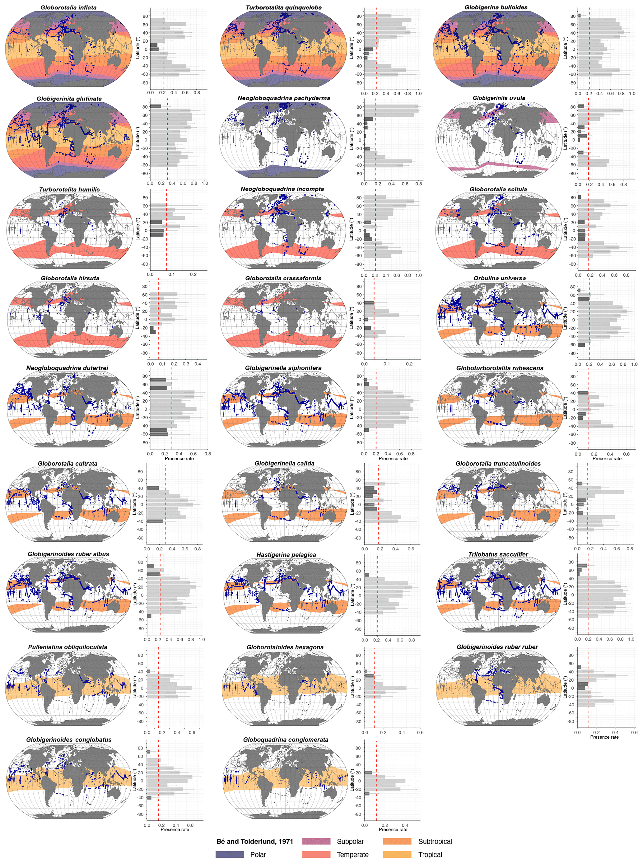
Figure 1 Latitudinal distribution patterns of planktonic foraminifera species. The left-hand side of each panel displays Robinson projection maps illustrating species presence (blue dots) and absence (grey dots) across global sampling sites (1970–2018), overlain on historical occurrence/presence provinces (coloured bands) as defined by Bé and Tolderlund (1971) and in related syntheses (Bé, 1977; Vincent and Berger, 1981) and aligned with the modern ecological concepts in Schiebel and Hemleben (2017), spanning global, polar, subpolar, temperate, subtropical, and tropical zones (from top to bottom panels). Adjacent histograms (right-hand side of each panel) show the presence rate of each species within 10° latitude bins. Dark-grey bars represent latitudinal bins where species are outside of their expected biogeographic province, while light-grey bars correspond to bins where species are within their expected habitats. The dashed red line denotes the species-specific threshold used to identify significant distribution patterns. G. uvula historical occurrence was taken from Schiebel and Hemleben (2017) and is flagged accordingly.

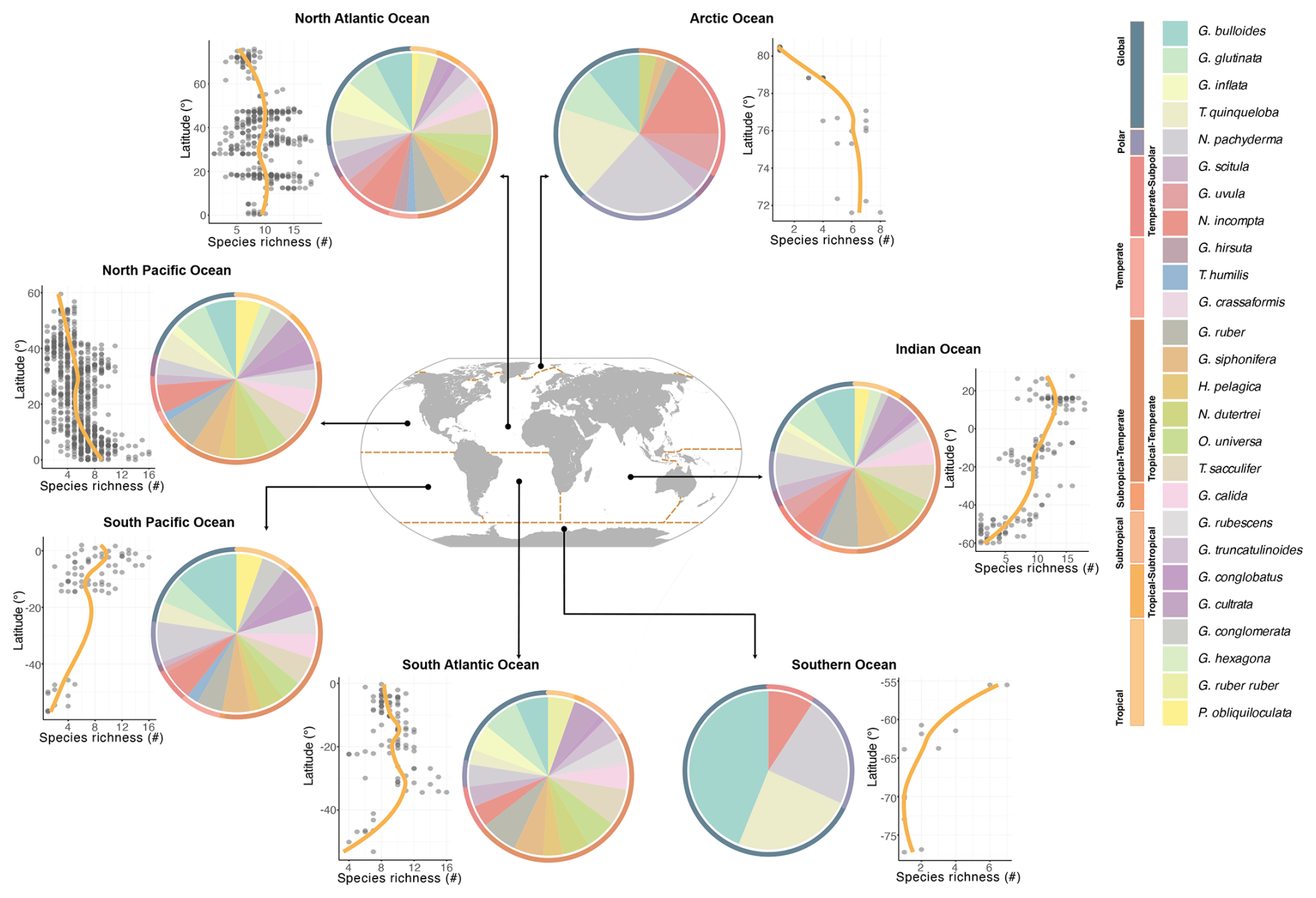
Figure 2 Biodiversity of modern planktonic foraminifera at the basin scale. Latitudinal diversity gradient displaying species richness as a function of latitude across different ocean basins and a comprehensive representation of modern PF diversity of major species within different ocean basins. Pie charts show the presence of species, and circles show the zones ranging from global to polar, subpolar, temperate, subtropical, and tropical. LOESS (yellow line) curves in cross-plots highlight the trend in species richness across latitudes.

To define the distribution patterns of the different PF species, we analysed their presence rates across latitudinal gradients for the period between 1970 and 2018 using solely the plankton net and pump data from the FORCIS database. The continuous plankton recorder (CPR) data were excluded from the maps in Fig. 1 and the presence rate calculations due to the disproportionately high number of zero (absence) records in the dataset, which could bias the latitudinal patterns. Species presence across latitudes was quantified using a binary presence–absence metric. First, the global sampling area was divided into 5° × 5° grid cells, and the presence of each species was recorded in each cell (presence = 1 if at least one sample in the cell contained the species; absence = 0 if sampled but not detected; unsampled cells = NA and excluded). These grid-level presence data were then aggregated into 10° latitudinal bins, and the presence rate P for each bin was calculated as the proportion of grid cells containing the species relative to the total number of equal-area grid cells in that latitudinal band, such that the presence rate reflects the proportion of occupied area within each latitudinal band rather than being biased by uneven sampling density using Eq. (3):

$$\begin{array}{}\text{(3)}& P={\displaystyle \frac{\mathrm{presence}\mathrm{count}}{\mathrm{presence}\mathrm{count}+\mathrm{absence}\mathrm{count}}}.\end{array}$$

Equation (3) is used to quantify species distributions across environmental gradients as it represents the probability of presence for a given species in a particular area (e.g. McGill et al., 2007; Gotelli and Ellison, 2004). Only grid cells where the number of absence and/or presence is equal to at least 1 were considered (grid cells without any observations were not considered).

To improve the robustness of the presence rate patterns, we excluded the outer edges of the species distribution, where data were sparse and more likely to reflect inconsistent occurrences. We quantified the variability in presence rate by calculating the standard error (SE) of the binomial proportion for each species. Presence rate was defined as the proportion of samples in which the species was detected relative to the total number of samples with valid species counts (Eq. 4):

$$\begin{array}{}\text{(4)}& \mathrm{SE}=\sqrt{{\displaystyle \frac{P\times (\mathrm{1}-P)}{\mathrm{presence}\mathrm{count}+\mathrm{absence}\mathrm{count}}}}.\end{array}$$

To define the distributional limits of each species, we established thresholds using the respective presence rates. The threshold T for each species was calculated as a value within the observed range of presence rates based on the minimum P_min and maximum presence P_max rates across all latitude bins (Eq. 5). Specifically, the threshold was set as follows:

$$\begin{array}{}\text{(5)}& T=P_{\min }+\mathit{\alpha }\times (P_{\max }-P_{\min }),\end{array}$$

where P_min is the minimum presence rate in all of the latitude bins (excluding zero); P_max is the maximum presence rate in all of the latitude bins; and α is a scaling parameter, which determines how much of the range between the minimum and maximum is used to define the threshold.

This approach is used to define biogeographical boundaries based on species presence probability and is often used in ecological modelling to define areas where a species is most likely to thrive (Elith et al., 2006). The threshold helps delineate areas where the species is present and ecologically viable. In addition, this threshold marks a point where the relationship between species occurrence and latitudinal bands is indicative of the overall distribution. To validate the selection of the alpha value for our threshold, a sensitivity analysis was conducted to systematically evaluate how different alpha values influence the identification of significant latitudinal bands across species. The alpha value, representing the scaling factor, was tested across a range of values, specifically 0.10, 0.15, 0.20, 0.25, and 0.30. For each species, we first calculated the minimum non-zero and maximum presence rates across latitudinal bands, followed by the computation of a threshold based on each alpha value using Eq. (5). Then, the number of bands that have a presence rate (P) above a certain threshold (T, number of significant bands) was calculated for each species and each alpha value (Figs. S1 and S2 in the Supplement).

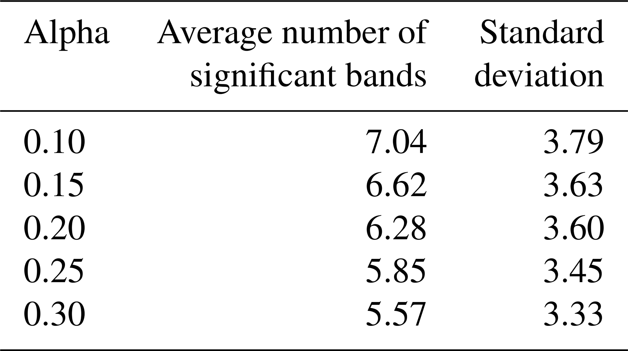
Subsequently, the calculated average number of significant bands across all species and the corresponding standard deviation for each alpha value were calculated (Table 1 and Fig. S2), providing a balanced trade-off between sensitivity (number of significant bands) and variability (standard deviation). The chosen threshold of the alpha value in this work is 0.20 since this identifies a moderate number of significant occurrence bands across species. This value strikes a balance between excluding the extremes (i.e. very low or very high presence rates) and capturing the stable, central part of the species' latitudinal presence distribution (Fig. S2). In other words, bands with presence rates just below this threshold are generally very weak (low bars), whereas those above them represent high presence rate values of each species' distribution. Thus, choosing α= 0.20 strikes an optimum balance between excluding noise at the extremes and preserving the main biogeographic signal.

Table 1 Sensitivity analysis of alpha values and their effect on the number of significant latitudinal bands across species.

Finally, to define biogeographic provinces, the Northern Hemisphere and Southern Hemisphere were divided into nine distinct provinces, comprising primary provinces (tropical, subtropical, temperate, subpolar, and polar), transitional provinces where these primary provinces overlap (tropical to subtropical, subtropical to temperate, tropical to temperate, and temperate to subpolar), and a category for ubiquitous species with global distributions (Table S2).

To address PF distribution changes in the pre-1970 time interval, species-specific presence rate patterns from the FORCIS database (1970–2018) were compared to the historical biogeographic provinces defined by Bé and Tolderlund (1971), as synthesised in Bé (1977) and Vincent and Berger (1981) and updated to modern ecological concepts by Schiebel and Hemleben (2017). Our approach identifies latitudinal preference zones where species' presence exceeds a defined threshold, representing areas of significant or maximum presence. These were then plotted with the historical biogeographic zones delineated by Bé and Tolderlund (1971) and other mentioned studies, focusing especially on the habitat of occurrence (Fig. 1). Bé and Tolderlund (1971) used the observed distribution and highest relative abundances of PF species along temperature and latitudinal gradients to describe their occurrence and/or tolerance biogeographic zones. Our approach captures zones of maximum presence without implying strict biogeographic exclusion outside of these zones. The compilation of works in this study, together with the observations from Bé and Tolderlund (1971) and the references therein, allows us to update the ecological preferences of each PF species using finer and higher data distributions (Figs. 1 and 5).

The robustness of species' biogeographic classifications is assessed using sensitivity maps combining presence–absence distributions with latitudinal presence rate histograms based on samples in which the entire assemblage was identified to the species level and samples where not all of the species were quantified (Fig. S3 and Table S4). Additional tests explore the spatial distribution of PF in samples collected with fine (≤ 200 µm) and coarse (> 200 µm) mesh sizes to account for different sampling strategies used in past projects (Fig. S4 and Table S4).

2.4 Assessment of PF species distributions and biodiversity in the contemporary global ocean

Biodiversity of PF in the contemporary ocean has been assessed by species richness (Fig. 2) from each sample of plankton net data in the FORCIS database, ranging from the sea surface (0 m) to the subsurface (> 200 m) ocean across all seasons from 1970 to 2018, spanning defined latitudinal bands (Fig. 1). The analyses have been specifically focused on 26 major species, using a “lumped” taxonomy as reviewed by the FORCIS consortium (Chaabane et al., 2023). To assess biodiversity per ocean basin, the abundance data from all samples within each basin were converted into relative abundance and computed for two diversity metrics (Figs. 2 and S6), (i) species richness and (ii) the Shannon diversity index (Shannon, 1948), using the R package “vegan” (Oksanen et al., 2022). Species richness is the presence of species at a specific site. The Shannon diversity index is given for each ocean basin and 10° latitudinal band (Fig. S6) using the following formula (Eq. 6):

$$\begin{array}{}\text{(6)}& H_{\mathrm{s}}=-{\sum }_{i=\mathrm{0}}^S{\mathit{\rho }}_i\cdot \log {\mathit{\rho }}_i,\end{array}$$

where s is the total number of species at a specific site, and ρ_i represents the relative abundance of the ith species. The Shannon diversity index provides a measure of diversity that takes into account both the number of species and their relative abundances in the community. A Shannon diversity index value of zero (0) indicates that there is only one species present (no diversity), whereas higher values indicate increasing species diversity, with both the number of species and the evenness of their abundances contributing to a more diverse community.

In addition, the latitudinal diversity gradient (LDG) of PF was explored for each ocean basin by analysing the variation in species richness across latitudes (Figs. 2 and S7). Data from various sampling locations were filtered to include only those with valid latitudinal and depth information (above 200 m water depth). The species presence-to-absence data were used to calculate species richness for each latitude. A LOESS smoothing curve of 0.7 span was applied to visualise the trend in species richness across latitudes (Fig. 2).

To assess biodiversity metrics and also to compute the presence and abundance of rare species in each ocean basin, a double-rarity approach was used. Any species was considered to be rare when below the 25th percentile (first quartile) with regard to both relative abundance and frequency of occurrence across all samples (Fig. S5). This dual-criteria method allows for a more robust identification of species that are not only locally rare in terms of abundance but also limited in their spatial distribution. Such a method accounts for both absolute numbers and restricted biogeographic presence, which is particularly relevant for assessing the role of rare species in population dynamics and regional diversity patterns. This approach has been used in ecological studies to better characterise the “long tail” of rare species and their contribution to ecosystem structure and functioning (e.g. Magurran and Henderson, 2003).

For each species i, the relative abundance was computed (Eq. 7):

$$\begin{array}{}\text{(7)}& {\stackrel{\mathrm{‾}}{A}}_{ij}={\displaystyle \frac{\mathrm{1}}{n_j}}{\sum }_{j\in P_i}^n{A}_{ij},\end{array}$$

where

• A_ij is the relative abundance of species i in sample j,

• P_i is the set of samples where species i is present, and

• n_i is the number of samples where species i is present.

The frequency of occurrence was calculated for each sample using Eq. (8):

$$\begin{array}{}\text{(8)}& F_j={\displaystyle \frac{n_j}{n}},\end{array}$$

where

• n_i is the number of samples where species i is present, and

• n is the total number of samples.

Species are defined as rare if both $\stackrel{\mathrm{‾}}{A}$ and F are below their respective 25th percentile thresholds (computed across all species).

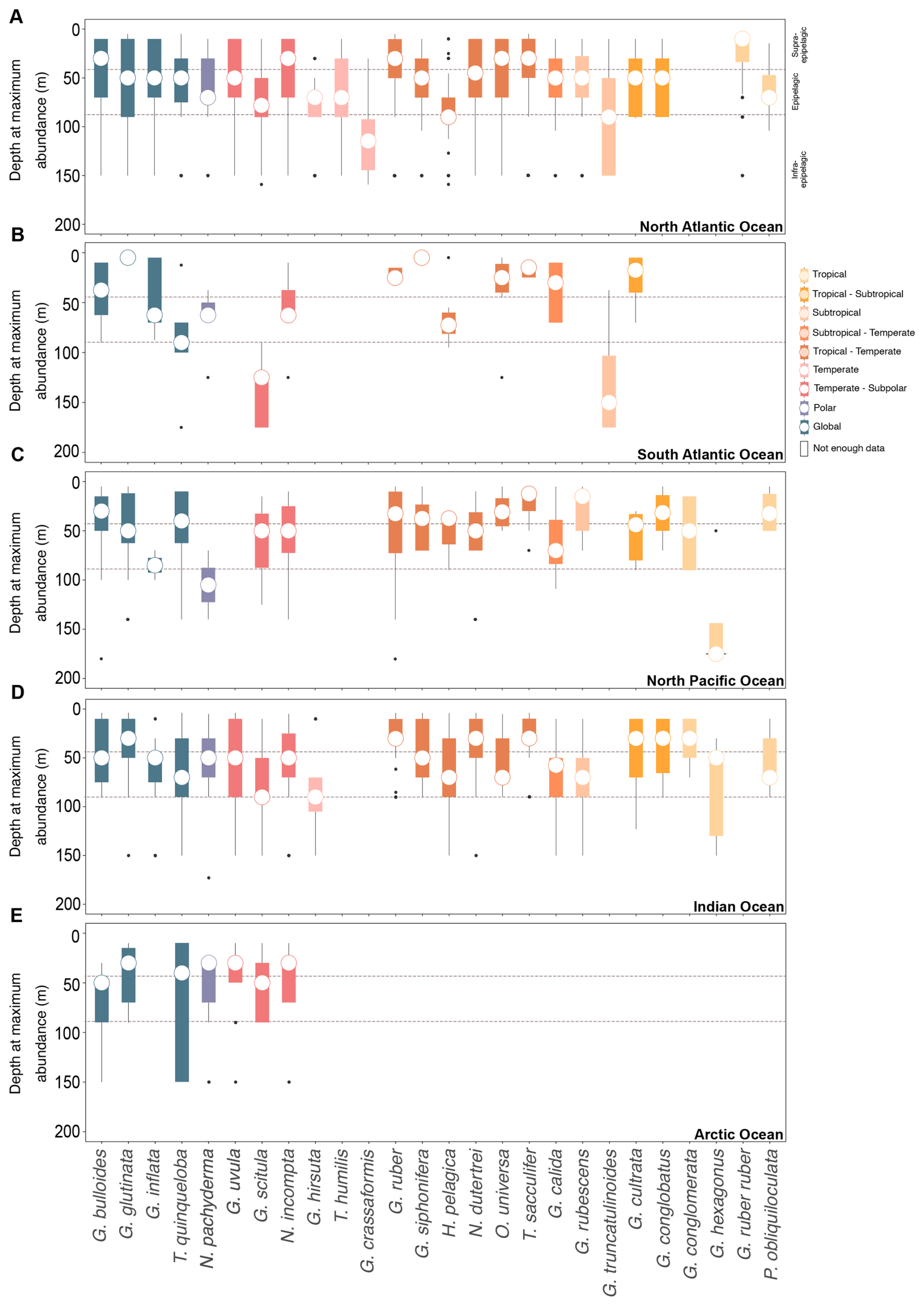
Figure 3 Vertical habitat preferences of planktonic foraminifera across various oceanic basins. The depth at the maximum abundance of PF gathered via plankton tows (multinet). The dataset encompasses the upper 200 m of the water column post-1970 in the (A) North Atlantic Ocean, (B) South Atlantic Ocean, (C) North Pacific Ocean, (D) Indian Ocean, and (E) Arctic Ocean. The species are organised from polar to tropical from left to right, with global species on the extreme left.

2.5 Average occurrence depth of modern PF

The depth habitats of the 26 main modern PF species across various ocean basins are derived from multinet samples from the upper 200 m of the water column. This depth range was chosen as it encompasses most of the habitat of PF species (Rebotim et al., 2017). All species counts obtained from samples obtained with plankton nets of varying mesh sizes were converted into absolute abundances and normalised at 100 µm in order to facilitate comparability of data (Chaabane et al., 2024b). For normalisation, the rather small 100 µm mesh size was chosen to include as much information provided in the aggregate dataset as possible. To further ensure data consistency, only depth profiles with at least four different depth intervals and similar sampling resolution (including consistent sampling depth intervals) during the spring and summer months are considered. From the selected datasets (n= 2388), the water depth at which each species exhibited maximum abundance per profile was calculated to identify the preferred water depth ranges of each species in the respective ocean basin (Fig. 3 and Table S5).

The average occurrence depth (AOD) of the 26 dominant species in the modern PF populations was determined by computing the abundance-weighted mean depth across sampled intervals within the upper 200 m of the ocean using multinet samples (Table 2). The calculation of both the species' number concentration within the depth intervals (measured in individuals per cubic metre) and the minimum and maximum AOD, as well as the associated standard error, follows the equation of Rebotim et al. (2017):

$$\begin{array}{}\text{(9)}& \mathrm{AOD}={\displaystyle \frac{\sum C_{i,j}\cdot D_i}{\sum C_{i,j}}},\end{array}$$

where C_i,jj is the abundance of the species in depth interval i at profile j, and D_i is the midpoint depth of interval i.

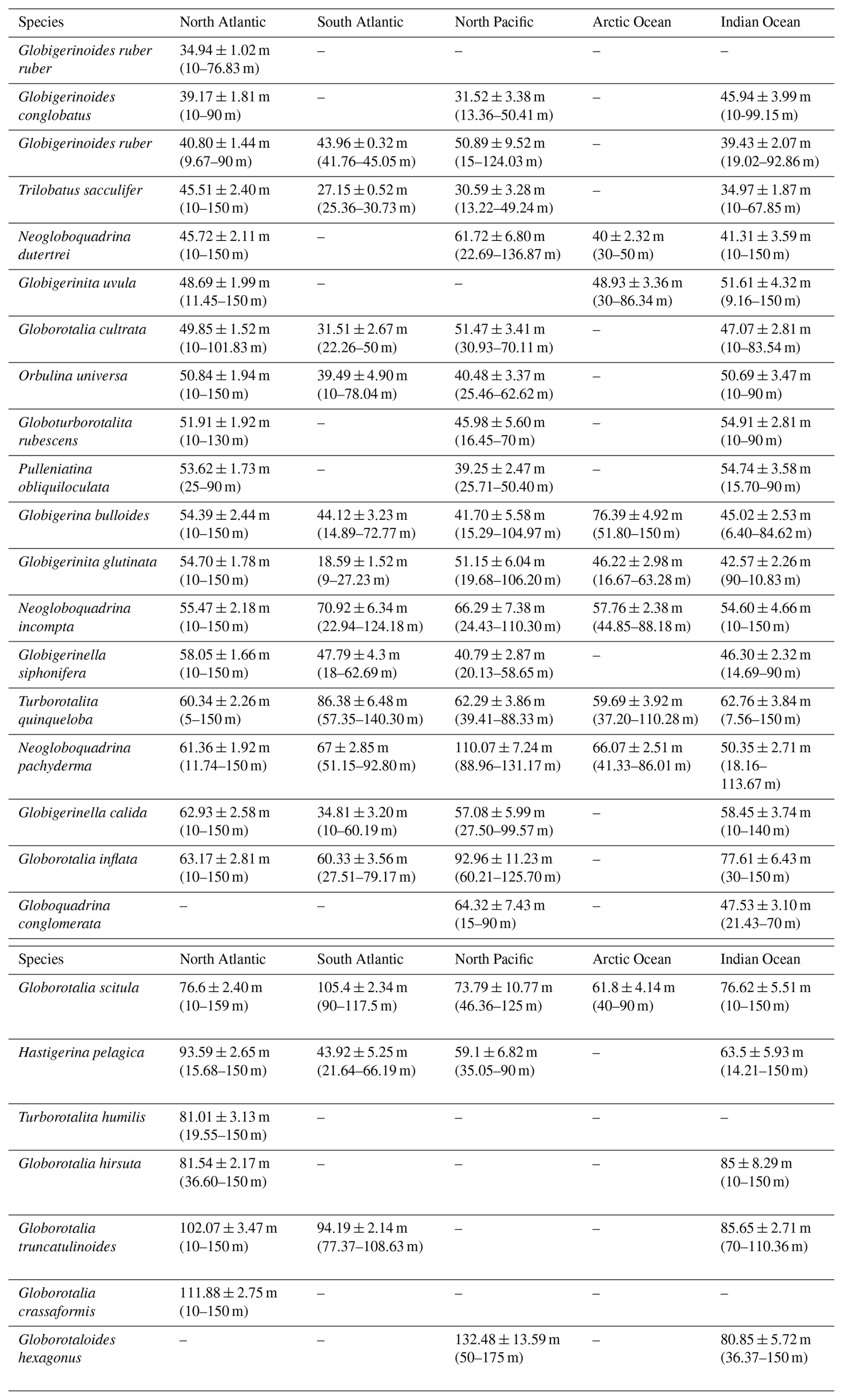
Table 2 Average (mean ± standard error) occurrence depth, as well as minimum and maximum average occurrence depths (in metres below the sea surface) of various PF species across different ocean basins. Each entry represents the calculated mean depth along with its associated standard error for a particular species within a specific ocean basin. The data reveal species-specific distribution patterns, with some species exhibiting notable variations in depth preferences across different basins.

The minimum and maximum AOD values correspond to the shallowest and deepest weighted mean depths observed among all profiles, reflecting the species' vertical habitat range:

$$\begin{array}{}\text{(10)}& {\displaystyle }{\mathrm{AOD}}_{\min }=\min j{\displaystyle \frac{\sum C_{i,j}\cdot D_i}{\sum C_{i,j}}},\text{(11)}& {\displaystyle }{\mathrm{AOD}}_{\max }=\max j{\displaystyle \frac{\sum C_{i,j}\cdot D_i}{\sum C_{i,j}}},\end{array}$$

where j indexes different sampling profiles.

AOD was only determined for profiles with at least four different depth intervals. Then, the species' depth habitat and the AOD were categorised into three distinct intervals (Meilland et al., 2021): supra-epipelagic (0–40 m), epipelagic (40–80 m), and infra-epipelagic (80–200 m).

To test among-basin differences in terms of the depth at the maximum abundance, we ran a one-way Welch ANOVA, with ocean basin as the factor (robust to unequal variances and unbalanced n, Welch, 1951), followed, when significant, by Games–Howell pairwise comparisons with the Benjamini–Hochberg false-discovery-rate control across basin pairs (Games and Howell, 1976; Benjamini and Hochberg, 1995). Species were included when ≥ 5 independent profiles were available in at least two basins. To compare the shape of the depth at the maximum abundance distributions among basins, we binned the depth at the maximum abundance into 10 m histograms (0–200 m) and computed Pearson correlations between basin-wise probability vectors, plotting a correlation heatmap for each species (Fig. S8).

2.6 Assessment of thermal preferences

To ascertain the thermal tolerance of individual PF species across different ocean basins, defined as the temperature range at which a species of PF can be observed, irrespective of its abundance, analyses were restricted to absolute abundance data from the plankton net normalised at 100 µm within the FORCIS database collected post-1970 from the top 100 m of the water column. Then, mean in situ temperatures (reanalysis at the time and at the water depth of PF sampling) were extracted from the Hadley EN 4.2.1 Reanalysis Data analyses g10 (Good et al., 2013) at a monthly spatial resolution of 1° × 1° and a vertical resolution comprising 42 standard depth levels, ranging from the sea surface to 5500 m (Figs. 4 and S9) for each sample closest to the 4D grid (latitude × longitude × depth × time). Within 0–200 m, EN4 levels occur at ∼ 5–185 m in ∼ 10–20 m increments. The mean temperature is calculated by averaging the minimum and maximum extracted temperatures at the month of the collection and the minimum and maximum sampled water depths for each profile. This minimum–maximum averaging assumes an approximately linear vertical gradient and does not capture fine-scale thermal structure. However, continuous high-resolution profiles were unavailable for many historical and remote samples. Therefore, our approach, applied uniformly across all data, was the only feasible way to generate homogenous thermal estimates. While this approach may not appreciate smooth small-scale variability, it is sufficient for defining broad species-level thermal tolerance patterns.

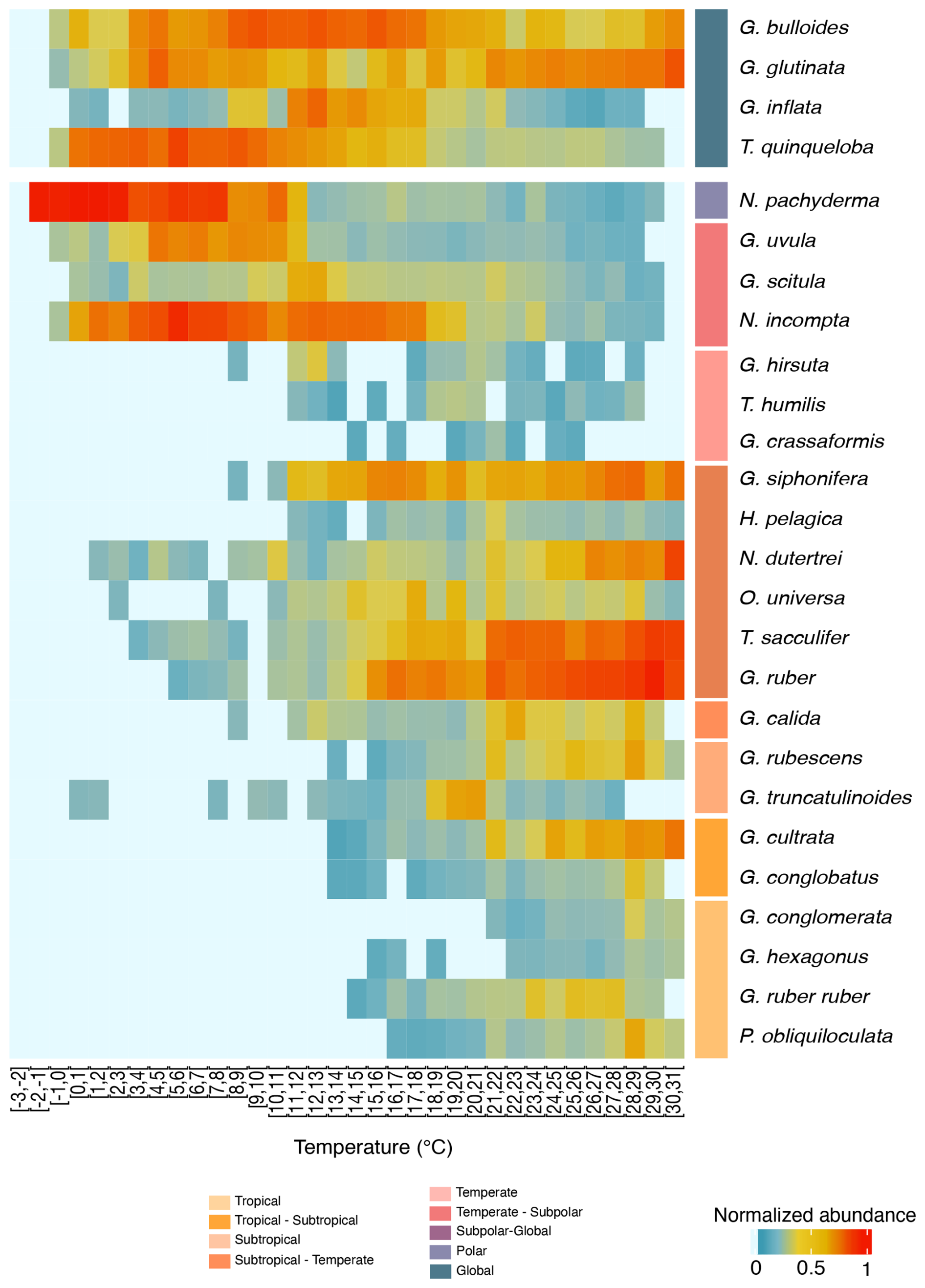
Figure 4 Temperature-related abundance variations of planktonic foraminifera. Heatmap presenting the normalised abundance of the most abundant planktonic foraminifera species from the FORCIS database (Chaabane et al., 2023). Data are from samples collected by plankton nets and pumps across the global ocean. Temperature bins are spaced at 1 °C intervals (x axis) and encompass the depth range of 0 to 100 m after 1970. Mean in situ temperatures are computed from minimum and maximum temperature values extracted from the Reanalysis Data Hadley EN 4.2.1 analysis g10 dataset, providing temperature information at a 1 × 1° resolution.

To generate a heatmap (Fig. 5), species abundances were normalised within each temperature bin (i) to account for variability and to facilitate inter-bin comparisons. Normalisation was performed using the following steps.

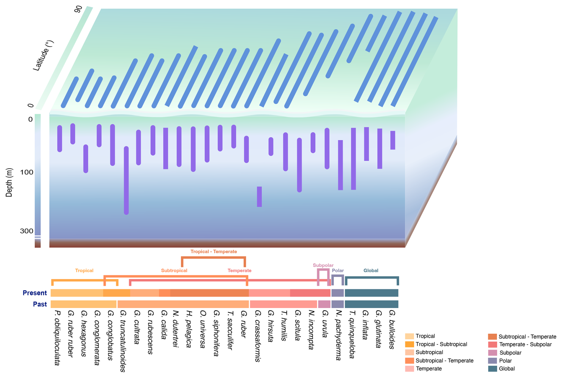
Figure 5 Schematic of latitudinal and water depth patterns of the global distribution of planktonic foraminifera. PF water depth habitats, latitudinal distributions, and temperature ranges of major species. Species are grouped by biogeographic province (post-1970) as proposed in this study (global, polar, subpolar–global, subpolar, subpolar–temperate, temperate, temperate–subtropical, subtropical, subtropical–tropical, and tropical oceans) and compared to the biogeographic provinces proposed by Bé and Tolderlund (1971) for samples obtained before 1970.

First, the raw abundance of each species (A_s,i) in a given temperature bin (i) was scaled using the following formula:

$$\begin{array}{}\text{(12)}& Z_{\mathrm{s},i}={\displaystyle \frac{A_{\mathrm{s},i}-{\mathit{\mu }}_i}{{\mathit{\sigma }}_i}},\end{array}$$

where μ_i is the mean abundance of all species in bin i, and σ_i is the standard deviation of species abundances in bin i. This approach centres the data around zero and scales by the variability within each bin, ensuring comparability across bins. Then, the scaled abundances (Z_s,i) were averaged across samples within each bin to compute the mean scaled abundance per species.

To ensure the robustness of the analyses on the thermal preferences of PF, we conducted a sensitivity test in which the entire thermal tolerance analysis was repeated using (i) the raw, uncorrected abundance data (Fig. S10) and (ii) only the subset of samples collected with mesh sizes of ≤ 200 µm (Fig. S11).

2.7 Statistics

All analyses were executed using R version 4.3.3 (29 February 2024). Data cleaning and import were facilitated by the tidyverse package, and ggplot (Wickham, 2016, Wickham et al., 2019) was employed for generating the plots. The abundance normalisation and scaling were implemented in R using the scale function within the dplyr workflow (Johnson and Wichern, 2007). The mutate_at function was applied to group the data by temperature bins and to scale the species abundances (Wickham et al., 2019). The LOESS smoothing curve is applied using the geom_smooth() function in ggplot2 (Wickham, 2016). To test among-basin differences in the depth at the maximum abundance, the purrr and rstatix packages were used (Wickham et al., 2023, Wickham and Henry, 2023; Kassambara, 2023).

3 Results

3.1 Latitudinal gradients and habitat specialisation in planktonic foraminifera

Planktonic foraminifera show latitudinal distribution patterns, averaged over the 1970–2018 time interval, with maximum diversity in the tropical and subtropical oceans (Figs. 1, 2, 5, and S7). In contrast, PF assemblages are less diverse within the polar zones, occupied (in terms of presence) mostly by Neogloboquadrina pachyderma (Figs. 1 and 4). However, a clear latitudinal presence rate gradient is not uniformly observed across all species. The presence rates (Eq. 3) of species reveal different distribution patterns for planktonic foraminifera across latitudes. Globorotaloides hexagonus and Globoquadrina conglomerata thrive in tropical zones (Figs. 1 and 4). Tropical to subtropical assemblages are characterised by Globigerinoides ruber ruber, Globoturborotalita rubescens, Pulleniatina obliquiloculata, and Globigerinoides conglobatus (Figs. 1 and 4). In subtropical and temperate zones, species such as Globigerinella calida, Trilobatus sacculifer, Neogloboquadrina dutertrei, Globigerinella siphonifera, Globigerinoides ruber, and Orbulina universa are frequently observed (Fig. 1). Subpolar to global species, such as Globigerinita uvula, reflect an ecological adaptability as they occur across a wide range of climatic zones (Fig. 1). Neogloboquadrina incompta, Globorotalia scitula, and Globorotalia hirsuta (mostly North Atlantic)  thrive in transitional environments between temperate and subpolar zones (Figs. 1 and 4). The polar species Neogloboquadrina pachyderma extends into subpolar waters (Fig. 3). Species with a global distribution include Globigerina bulloides, Globigerinita glutinata, Turborotalita quinqueloba, and Globorotalia inflata, spanning multiple climatic zones and reflecting their ecological versatility (Figs. 1 and 3). Even when the analyses were restricted to samples in which the entire assemblage was counted at the species level (Fig. S3), the global latitudinal distribution patterns of PF remain consistent with those observed using the full dataset (Figs. 1 and S3). This consistency reflects the relatively low number of samples in which not all species were counted, indicating that the excluded samples have a minimum impact on the overall biogeographic patterns. Similarly, the distributional patterns of PF observed in samples collected with a mesh size ≤ 200 µm are largely consistent with those derived from the global dataset (Fig. S4).

The highest PF diversity is observed in the tropical to subtropical North Atlantic, Pacific, and Indian oceans, with a maximum species richness ranging between 16 and 19 (Figs. 2 and S7). In contrast, the lowest diversity is recorded in the Arctic and Southern oceans, with a mean richness of only three to four species (Figs. 2 and S7). Accordingly, the Pacific, Atlantic, and Indian oceans host globally distributed species and those adapted from tropical to temperate zones. Low numbers of species, on the other hand, are primarily found in the Arctic and Southern oceans. Certain species and subspecies exhibit distinct regional distributions, such as G. ruber ruber, which is exclusive to the Atlantic Ocean, while G. conglomerata and G. hexagonus are confined to the Indian and Pacific oceans (Figs. 1 and 2).

The Shannon diversity index reaches its peak in the low latitudes (Fig. S6), specifically between 30° S and 30° N, exhibiting values between 1 and 2. Highest Shannon diversity index values within this latitude range have been recorded in the Atlantic and Pacific oceans. There is a noticeable decrease in the Shannon diversity index with increasing latitude south and north of 30°. In the mid-latitudes, reaching from 30 to 60° (north and south), the Shannon diversity index ranges from 0.5 to 1.5. In contrast, at the high latitudes, exceeding 60° N and 60° S, Shannon diversity index values are consistently lower than 1 (Fig. S6).

3.2 Average occurrence depth

The majority of PF species are present at an AOD (Table 2) and a depth at maximum abundance (Figs. 3) in the upper epipelagic zone, i.e. the upper 100 m of the water column. In the supra-epipelagic level (0–40 m), species such as G. ruber ruber and G. conglobatus are found. Species like G. ruber, T. sacculifer, N. dutertrei, G. uvula, G. cultrata, O. universa, G. rubescens, P. obliquiloculata, G. bulloides, G. conglomerata, G. glutinata, G. siphonifera, G. calida, G. inflata, and G. scitula are recorded in the epipelagic zone at 40–80 m (Table 2). Within the infra-epipelagic domain (80–200 m), multiple species are observed, including T. humilis, G. hirsuta, G. truncatulinoides, G. crassaformis, and G. hexagonus, with varying AOD across different regions, suggesting a slightly variable preferential depth habitat subjected to changes in depth distribution.

Overall, globally distributed species maintain the same depth habitat across the Atlantic, Indian, Pacific, and Arctic oceans (Fig. 3). The South and North Atlantic host diverse epipelagic species such as T. sacculifer, G. ruber, and G. ruber ruber, predominantly living in the upper 100 m. Infra-epipelagic-dwelling species include, for example, G. truncatulinoides and G. crassaformis, with a depth of maximum abundance extending to below 150 m water depth. In the Arctic Ocean, PF assemblages are dominated by non-spinose species such as N. pachyderma, G. glutinata, G. uvula, T. quinqueloba, G. bulloides, N. incompta, and G. scitula, typically the upper 100 m water depth (Figs. 3 and 5). In the North Pacific Ocean, the distribution patterns largely align with observations from the North Atlantic, with a few noteworthy differences (Fig. 3). In the North Pacific, most PF species reach maximum occurrence within 0–100 m, as in the North Atlantic, but N. pachyderma attains a deeper depth of maximum abundance in the Pacific than in the Atlantic and, correspondingly, occupies colder waters there; in the North and South Atlantic, the species' peaks occur at shallower depths and span a broader, warmer temperature range (Figs. 3 and S9). In the North Pacific, N. pachyderma has also been occurring in slightly deeper waters (often below 100 m) than in the North Atlantic, southern Indian, and Arctic oceans (mostly above 100 m; Fig. 3), while G. bulloides is found at greater depths in the Arctic Ocean (often below 50 m) compared to in the other ocean basins (mostly above 50 m; Fig. 3). While the majority of species reside in the upper 100 m of the water column, certain species such as G. conglobatus and G. conglomerata prefer water depths above 50 m. Conversely, species like G. calida, G. rubescens, and H. pelagica inhabit the lower mixed layer between 50 and 100 m water depth. Species like G. hirsuta and G. scitula may still occur in the subsurface layer below 100 m (Fig. 5). Though AODs of species are mostly consistent across the different basins (Fig. S8), except for a few species like T. sacculifer and G. siphonifera , which live at shallower depths in the North Pacific and Indian oceans, and G. inflata, which lives, on average, at deeper depths in the North Pacific and Indian oceans than in the Atlantic Ocean.

3.3 Temperature tolerance of planktonic foraminifera

Planktonic foraminifera are observed at temperatures spanning the full open ocean range, from about −2 to 31 °C (Figs. 4, S9, S10, and S11). The thermal tolerance of PF is defined as the range of seawater temperatures at which a given species has been observed. Overall, species' temperature tolerance ranges are between 10 and 25 °C. Several species are shown to live in the warmer temperatures (31 °C) of our dataset, particularly in tropical, subtropical, and subtropical-to-temperate assemblages. However, the true upper thermal limits of these species may exceed this value as our data do not include observations at higher temperatures (Schiebel and Hemleben, 2017). Tropical species occur from 14 to 31 °C, subtropical species occur from 12 to 31 °C, and subtropical-to-temperate species occur from 3 to 26 °C. Temperate species range from 8 to 25 °C, temperate-to-subpolar species range from 0 to 21 °C, subpolar-to-global species range from 0 to 18 °C, and polar species range from −2 to 11 °C (Figs. 4 and S9).

Globigerinella calida mostly occurs in warm water (mostly subtropical) between 20 and 30 °C in the North Atlantic Ocean but has been frequently observed at temperatures as low as 12 °C (Fig. 4). The polar to subpolar species N. pachyderma with temperature preferences around 2 °C (Fig. S9) frequently occur in waters of up to 11 °C and have been reported from waters as warm as 30 °C (Figs. 4 and S9). Finally, species with a global distribution, such as G. bulloides, G. glutinata, and T. quinqueloba, exhibit a high level of tolerance over an extensive temperature range (Fig. 4). These findings show the capacity of PF individuals to endure a wide range of thermal environments.

4 Discussion

4.1 Latitudinal distribution preferences of planktonic foraminifera

The distribution of PF largely follows latitudinal patterns driven by sea surface temperature (SST) and matches marine biogeographic provinces (e.g. Bradshaw, 1957; Bé and Tolderlund, 1971; Hemleben et al., 1989; Schiebel and Hemleben, 2005; Kucera, 2007; Longhurst, 2007; Spalding et al., 2007). The tropics and subtropics are primary realms for warm-water PF species such as G. ruber ruber, P. obliquiloculata, G. conglobatus, and G. conglomerata (Fig. 1), confirming the previously established SST-mediated distribution patterns documented in pre-industrial records (Rillo et al., 2022; Jonkers et al., 2019). Species like G. bulloides and G. glutinata have been globally distributed from pre-industrial to modern times and thrive across diverse marine environments (Figs. 1, 2, and 4). Species such as G. bulloides are abundant in eutrophic conditions associated with upwelling or spring blooms (Thiede, 1975; Kroon and Ganssen, 1988; Schiebel et al., 1995; Schiebel and Hemleben, 2000; Darling and Wade, 2008; Conan and Brummer, 2000; Seears et al., 2012). The tolerance to a wide range of ecological conditions may be explained by the fact that different genotypes, encompassed within classical morphotypes of G. bulloides, exhibit different ecological preferences, leading to a broad overall tolerance (Morard et al., 2013, 2024; Darling et al., 2017). Most PF morphospecies combine more than one genotype and “cryptic species” with allopatric occurrences, indicating speciation at the regional scale (e.g. Darling and Wade, 2008; Morard et al., 2024).

For example, both morphospecies G. glutinata and G. bulloides include some 4 to 10 genotypes, respectively, with particular regional occurrences and narrower temperature ranges than the entire morphospecies (Darling et al., 2000; Darling and Wade, 2008; Ujiieì and Lipps 2009; Seears et al., 2012; Morard et al., 2013; André et al., 2013, 2014). Some occurrences of N. pachyderma in lower-latitude upwelling areas (Darling et al., 2000; Darling and Wade, 2008) affirm its adaptability and competitive advantage through opportunistic strategies, paralleling its success in polar-to-subpolar waters, indicating a r-selected life strategy. This strategy is characterised by rapid reproduction and high offspring numbers to facilitate survival in an environment with short productive seasons like the polar summer or seasonal upwelling (Schiebel and Hemleben, 2005; Jonkers et al., 2010; Ivanova et al., 1999; Meilland et al., 2023).

In comparison to the seminal works of Ruddiman et al. (1970) and Bé and Tolderlund (1971), our observations from the FORCIS database show that species previously considered to be subtropical, temperate, and subpolar have recently also been found at higher latitudes, suggesting that their habitat has expanded polewards (Chaabane et al., 2024a). The biogeographic provinces provided by Bé and Tolderlund (1971) are used here as a historical baseline, although these are based on data produced with different methodologies such as larger mesh sizes. Consequently, the resulting differences in latitudinal expansion and water depth intervals should be considered to be relative indications of distributional shifts rather than absolute precise zonation reassignments. Notably, tropical species have been transitioning to subtropical zones, subtropical species have been transitioning to temperate regions, temperate species have been transitioning to subpolar areas, and subpolar species are expanding into polar to global latitudes (Figs. 1 and 5 and Table S1). Similar shifts have been observed in distributional patterns that began emerging in the last deglaciation, extending through pre-industrial times and over the last century. During the last deglaciation, PF assemblages rapidly responded to warming by shifting polewards (Strack et al., 2022). Yasuhara et al. (2020) showed that this trend persisted into the pre-industrial time. Over the last century, new patterns of assemblages emerged (Chaabane et al., 2024a; Strack et al., 2022). Diversity increased at higher latitudes, while PF abundances, particularly in subtropical species, showed a marked decline (Chaabane et al., 2024a). This underscores the broader implications of global warming on marine biogeography. As shown earlier, species appear to colonise new suitable habitats in response to changing environments rather than adapting to locally changing conditions (Chaabane et al., 2024a; Benedetti et al., 2021; Jonkers et al., 2019; Strack et al., 2022).

The post-1970 data (FORCIS database) also reveal sporadic occurrences of tropical and subtropical species in polar regions, although in limited numbers. Species like G. calida and G. rubescens do now frequently occur at temperate rather than subtropical latitudes (Figs. 4 and S9), which may be episodic or may follow a systematic trend. Notably, species such as N. dutertrei, G. calida, and T. sacculifer, typically associated with specific thermal and geographic ranges (Bé, 1982), exhibit distinct distribution patterns out of their pre-1970 distribution. These species, traditionally associated with subtropical waters, are now frequently being observed in temperate zones of the North Atlantic Ocean, which may indicate poleward extension of their biogeographic zones or adaptation to new ecological niches (Chaabane et al., 2024a). Similarly, G. uvula, once predominantly found in subpolar waters, may establish a more global presence (Fig. 1). Overall, our analyses indicate compositional shifts before and after 1970 assemblages, with medium-sized species such as G. glutinata exhibiting broader spatial distributions than in pre-1970 records, where this was occurring globally, with a warm-water preference (Table S1; Parker and Berger, 1971; Bé and Tolderlund, 1971). In general, smaller species may offer specific biological advantages in a changing environment (Schmidt et al., 2004; Chernihovsky et al., 2020) by having lower energy demands than larger species, hence making them less vulnerable to environmental change (Burke et al., 2025). The presence of substantial populations of species such as G. conglobatus at low to middle latitudes and G. uvula at higher latitudes, which were not reported from PF assemblages before 1970, underscores the profound shifts occurring within marine ecosystems (Beaugrand et al., 2003).

4.2 Longitudinal changes in planktonic foraminifera assemblage patterns

The longitudinal patterns in the biogeography of PF are intricate when examining the post-1970 dataset of the comprehensive FORCIS dataset. In this study, we hypothesise that the high PF diversity in the North Atlantic across a wide range of temperatures and transportation of PF, notably by the Gulf Stream and North Atlantic Current, exert substantial influence on the distribution of species from the southwest to the northeast (Ingvaldsen et al., 2021; Polyakov et al., 2020, 2017; Fig. S9).

The tropical and subtropical Indian Ocean, with its monsoon-driven circulation (Schott and McCreary, 2001), presents a different case of regional and temporal complexity. Adjacent seasonal upwelling cells and stratified conditions in the subtropical gyre result in mixed assemblages of global and tropical to subtropical species, such as G. bulloides, G. conglobatus, and G. conglomerata, and temperate species like G. hirsuta (Figs. 2 and S9) (Conan and Brummer, 2000; Ivanova et al., 1999; Peeters et al., 1999; Brummer and Kroon, 1988; Schiebel et al., 2004).

The North and South Pacific exhibit PF distribution patterns, which are characterised by upwelling-related species in the eastern basins and tropical and subtropical species in the western basin. This pattern is affected by interannual changes related to the El Niño–Southern Oscillation (ENSO) from the eastern to western equatorial Pacific (Yamasaki et al., 2022). The conspicuous distribution of either warm-water- or cold-water-adapted species in the eastern South Pacific (Fig. S9) may reflect the regional and seasonal upwelling conditions off North and South America versus the oligotrophic conditions of the South Pacific subtropical gyre.

Finally, the observed distribution along longitudinal gradients in the modern oceans may be attributed to multiple factors including anthropogenic influences like ocean warming and consequent changes in surface ocean circulation, stratification, and nutrient dynamics, as well as ocean acidification (Orr et al., 2005).

4.3 Vertical distribution of planktonic foraminifera

Depth habitats of 26 modern PF species from all major ocean basins were determined using multinet data collected from the upper 200 m of the water column. Most PF species are confined to the uppermost 100 m of the water column from the supra-epipelagic to the epipelagic zones (Figs. 3 and 5), which includes the surface mixed layer and euphotic zone (e.g. Schiebel and Hemleben, 2017, and references therein). This preference for surface waters remains consistent across various ocean basins, albeit with variations in species composition. For instance, in this study, in the North Atlantic Ocean, species such as G. ruber ruber, P. obliquiloculata, and G. calida were, on average, found at AODs of 35, 53, and 63 m, respectively, compared to at 40, 45, and 73 m, respectively, as found by Rebotim et al. (2017). In the South Atlantic Ocean, G. cultrata, and O. universa were observed at 31 and 39 m, respectively, in this study, and at 39 and 30 m, respectively, by Lessa et al. (2020). In the Pacific Ocean, G. hexagonus was found at 132 m in this study compared to at the shallower depth reported in Davis et al. (2020). In the Indian Ocean, N. pachyderma and N. incompta were recorded at 50 and 55 m, respectively, in this study and between at 40 and 60 m by Meilland et al. (2018). Across basins, species' AOD differences are small and lie within the same vertical horizon of the water column (above, within, or below the thermocline); dispersion overlaps broadly among basins, and, consistently with our formal tests (Welch ANOVA with Games–Howell), we find no evidence for systematic inter-basin differences in vertical habitats (Fig. S8).

Species like G. bulloides exhibit a wide ecological niche, which may be attributed to different ecological niches of the different genotypes in the different global ocean basins discussed before (Berger, 1969; Watkins et al., 1998; André et al., 2014; Mallo et al., 2017; Morard et al., 2024). Overall, higher abundances of G. bulloides are related to enhanced nutrient concentrations and algal prey under upwelling conditions and seasonal algal blooms (Cifelli, 1974; Thiede, 1975; Schiebel and Hemleben, 2000). Across basins, the vertical position of G. bulloides seems to track food supply. It is shallower where surface layer phytoplankton production is elevated and deeper where export peaks below the thermocline or where mixed layers are deeper, in line with its trophic strategy (Schiebel and Hemleben, 2017; Meilland et al., 2020; Tell et al., 2022; Fig. 3).

A narrow depth distribution of species, such as the one observed in G. ruber and T. sacculifer, mostly in the epipelagic zone (< 60 m) in the tropical and subtropical ocean, may primarily be attributed to their photo-symbionts, which leave them restricted to certain light regimes (Spero and Lea, 1993; Gastrich, 1987; Hemleben et al., 1989). This suggests a finely tuned adaptation to surface and subsurface waters and underscores the sensitivity of the photo-symbiont-bearing species to changes in light conditions, which impacts their potential response to environmental change.

Most PF species show a rather variable depth distribution ranging from 30 to 70 m, on average, from the epipelagic to infra-epipelagic zone, such as O. universa and G. rubescens in the northeastern and southeastern Atlantic (Fig. S9) (Field, 2004; Bé and Hamlin, 1967; Kemle-von Mücke and Oberhänsli,1999). Neogloboquadrina incompta consistently occupies depths between 40 and 70 m (Fig. S9; Table 2). The presence of temperate species like G. hirsuta at varying depths hints at a wide ecological niche, potentially in response to seasonally changing hydrologic and trophic conditions (Schiebel and Hemleben, 2017). In the Indian Ocean, the depth distribution of species including G. conglobatus and G. conglomerata possibly results from monsoon-driven changes in surface water mixing versus stratification, nutrient availability, and alimentation of the PF (Schiebel et al., 2004; Morey et al., 2005).

The presence of species with a wide depth distribution from the sea surface and across the thermocline (supra-epipelagic to epipelagic zone), such as N. dutertrei, G. calida, G. inflata, H. pelagica, G. glutinata, T. humilis, N. pachyderma, G. scitula, and T. quinqueloba, highlights the adaptability to varying environmental conditions (Schiebel and Hemleben, 2017). Species like G. inflata and T. humilis exhibit a significant variability in their depth distribution (Fig. S8), which could be due to seasonal variations in the thermocline, reflecting the complex interplay between hydrographic (e.g. fronts) and ecological factors that determine their vertical habitat in the upper 100 m, and species living in the infra-epipelagic zone (below 100 m) (Fairbanks et al., 1980; Schiebel et al., 2001; Lončarić et al., 2006). Globorotaloides hexagonus, a possible indicator of oxygen-deficient conditions in the water column, has mainly been reported from shallow sub-thermocline depths in the North Pacific (Davis et al., 2021) and the (northern) Indian Ocean (Schiebel et al., 2004) (Figs. 1 and 3).

Subsurface-dwelling species, such as G. scitula, G. crassaformis, and G. truncatulinoides, have variable depth distributions typically below the seasonal thermocline (infra-epipelagic zone) during most of their post-juvenile ontogeny at a depth horizon that receives the prime export flux of matter from the overlying productive surface ocean (Bé and Hamlin, 1967; Kemle-von Mücke and Oberhänsli, 1999; Schmuker and Schiebel, 2002). The distribution ranges of these subsurface-dwelling species may indicate their adaptation to an alimentation based on a sufficient amount of organic matter settling out of the productive surface ocean. Accordingly, the regional distribution of the subsurface-dwelling species may also shift along with changing biological production and surface marine trophic conditions.

5 Conclusions

A comprehensive update of the global distribution, vertical habitat, and thermal tolerance and diversity of planktonic foraminifera (PF) in the modern (post-1910) oceans has been facilitated by the FORCIS database. Analyses confirmed that PF exhibit a persistent preference for the upper 100 m, likely driven by light and food availability. Modern PF span a wide temperature tolerance, ranging from −2 to 31 °C, which includes the entire temperature range of the modern oceans, underlining the eurythermal nature of these microplankton. At the species level, thermal niches are as wide and indicate that environmental parameters other than temperature affect their presence. These parameters may be the quantity and quality of prey, as well as light in the case of symbiont-bearing species.

While highly diverse PF assemblages at tropical and subtropical latitudes corroborate established latitudinal distribution patterns, species that appeared to be confined to lower latitudes before 1970 are now being described at higher latitudes. In addition, medium-sized species increased in number over all latitudes from the tropical to polar oceans, which is particularly clear from analyses of a vast amount of data from the eastern North Atlantic.

Despite their broad tolerance to varying environmental conditions, PF may be affected by changes in the marine environment, such as acidification, deoxygenation, and food availability, potentially leading to changes in population dynamics and PF assemblages. The PF biogeography presented in this study provides a nuanced understanding of PF diversity and distribution and underscores their value as paleoceanographic archives and proxies for a better understanding of the ongoing climate and ocean change.